This guide describes Flopsar Workstation usage.
1. Workstation Installation
Flopsar Workstation is a GUI client of the Flopsar environment.
Installation is straightforward, just copy the workstation-2.4.zip file to your machine and uncompress it. Next, run a workstation script from bin directory.
Note
You should have your Java environment set before you try to run the workstation application.
2. Accessing Flopsar Environment
When you execute the above command a login window Fig. 2.1 should appear.
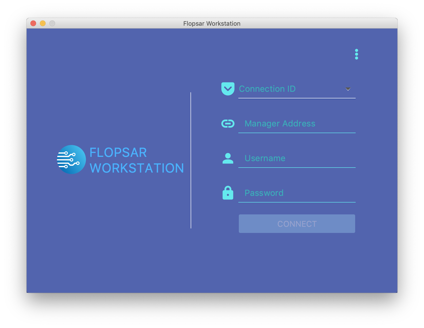
Fig. 2.1 Workstation Login: Remote Access
If you want to connect to some remote manager, select the Remote radio button. If you want to access your local copy of some database, select the Local radio button.
2.1. Remote Access
If you run workstation for the first time, the Connection ID combo box control is empty. In order to connect to your manager instance, you must specify some connection identifier (label) and input manager socket address in the form host:port. You must also provide your credentials and then click the Connect button. When you log to the manager instance successfully, the login window disappears and the main application window Fig. 3.3 appears instead. After a successful connection, your connection data are stored locally so that next time you start the application, the combo box will be filled with this stored connection information.
Important
Default credentials when using Flopsar Internal Authentication are as follows: the username is admin and the password is flopsar.
2.2. Local Access
In order to access your database locally, you just need to get the archive file from a selected database instance and copy it to your local disk. Next, click the option menu in the login window Fig. 2.1 and then select the Local item. Select either Storage or Archive File option and click on the … button to point to the database directory of the archive file, respectively. Next, click the CONNECT button.
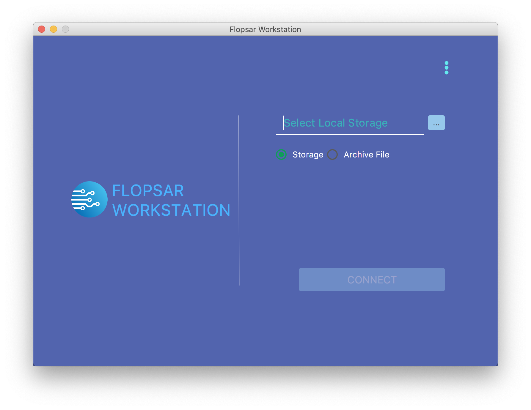
Fig. 2.2 Workstation Login: Local Access
3. Start Page
After you logged to the application, you should see its start page Fig. 3.3. There is a list of available queries you can make to the databases.
At the bottom, there is your current connection information to your manager and the number of connected databases. On the right side, there is a memory usage information of the application.
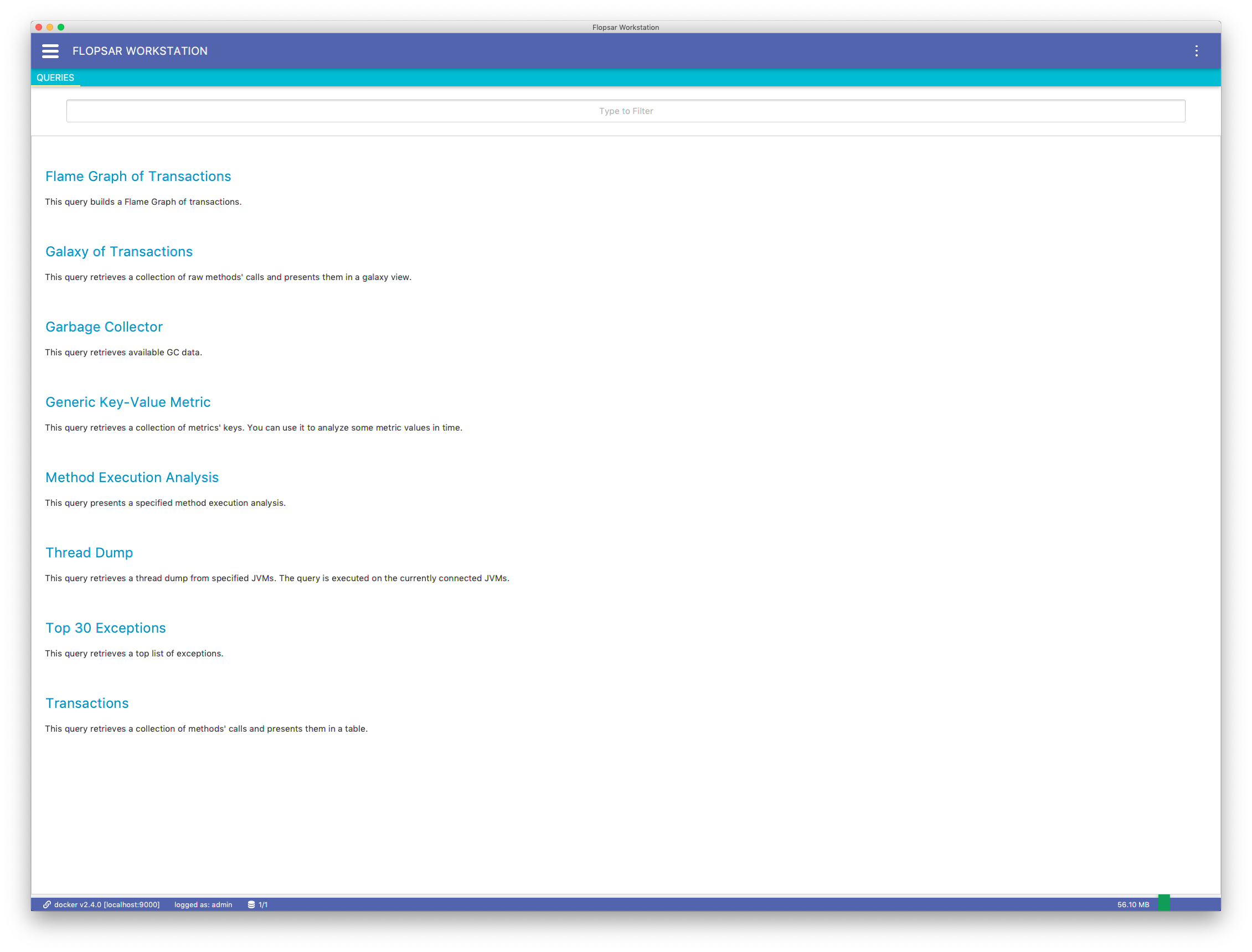
Fig. 3.3 Workstation: Start Page
If you access your local storage, you do not see the same workstation functionalities as in the remote access. That is because you do not connect to any manager instance, and the workstation runs in a viewer mode. At the bottom, there is a current local storage identifier and the number of connected databases (only one in this case). In both cases (remote and local), if you click the database icon, the pop-up Fig. 3.4 will appear with a list of databases. The list contains databases your manager is aware of. The list entries have socket addresses and versions of the databases. There is a link icon, at the beginning of each entry, which denotes a connection status. If the link is green, then the corresponding database connection is established. The link turns red if the connection is lost or does not exist.
Note
In case of local access, the database address is always localhost.
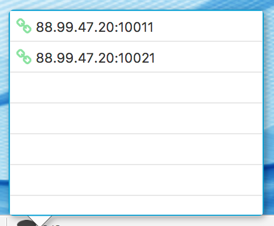
Fig. 3.4 Connected Databases
You can switch between different contexts by clicking the hamburger menu in Fig. 3.3. A drawer Fig. 3.5 will appear with a list of contexts. In order to manage your configurations click the CONFIGURATIONS (see Configurations for details). The AGENTS leads to a view where you can explore all the available agents (see Agents for details). The GALAXIES will take you to a view where you can manage your galaxies (see Galaxies for details).
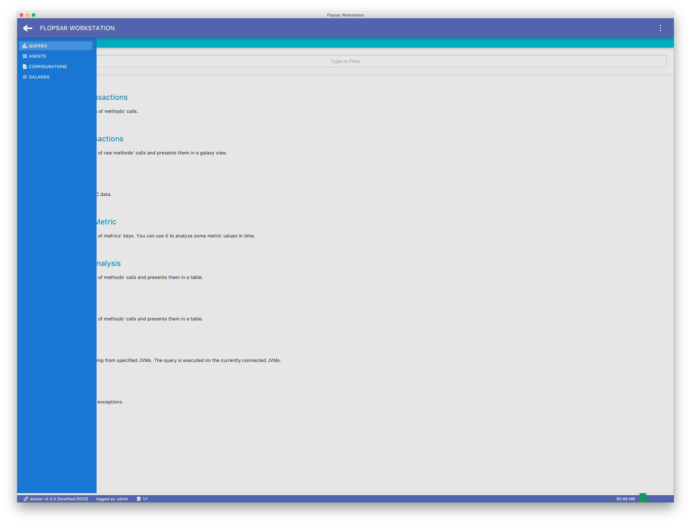
Fig. 3.5 Workstation: Start Page Menu
4. Settings
workstation stores its settings locally, on the machine it runs on. It makes use of Java Preferences API to store its configuration. The physical location of the settings depends on a platform the workstation runs on.
When you exit the application, it stores its current settings. These settings include the main application window size, some tables columns width, galaxy colors and the like.
4.1. General
By default, all the workstation logs are stored in a user home directory. This can be changed in the preferences window Fig. 4.2, where you can set both the logger level and the logs location. The logging levels are defined in Logging.
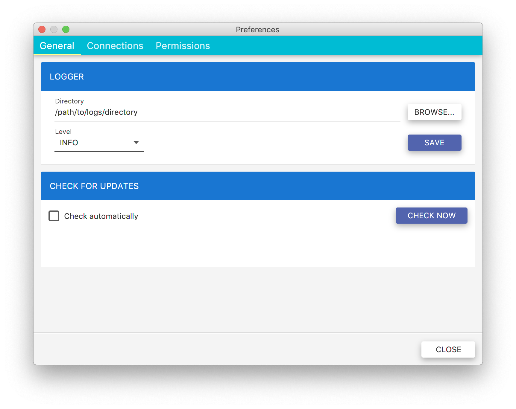
Fig. 4.2 Preferences: General
You can also check if there is a new Flopsar version available. In order to check it, just click the CHECK NOW button. If you enable the Check automatically, then whenever you start the workstation, it will check for updates automatically.
4.2. Connections
Besides the layout settings, your manager connections information is also stored in these settings. You can either edit or delete these connections in the preferences window Fig. 4.3.
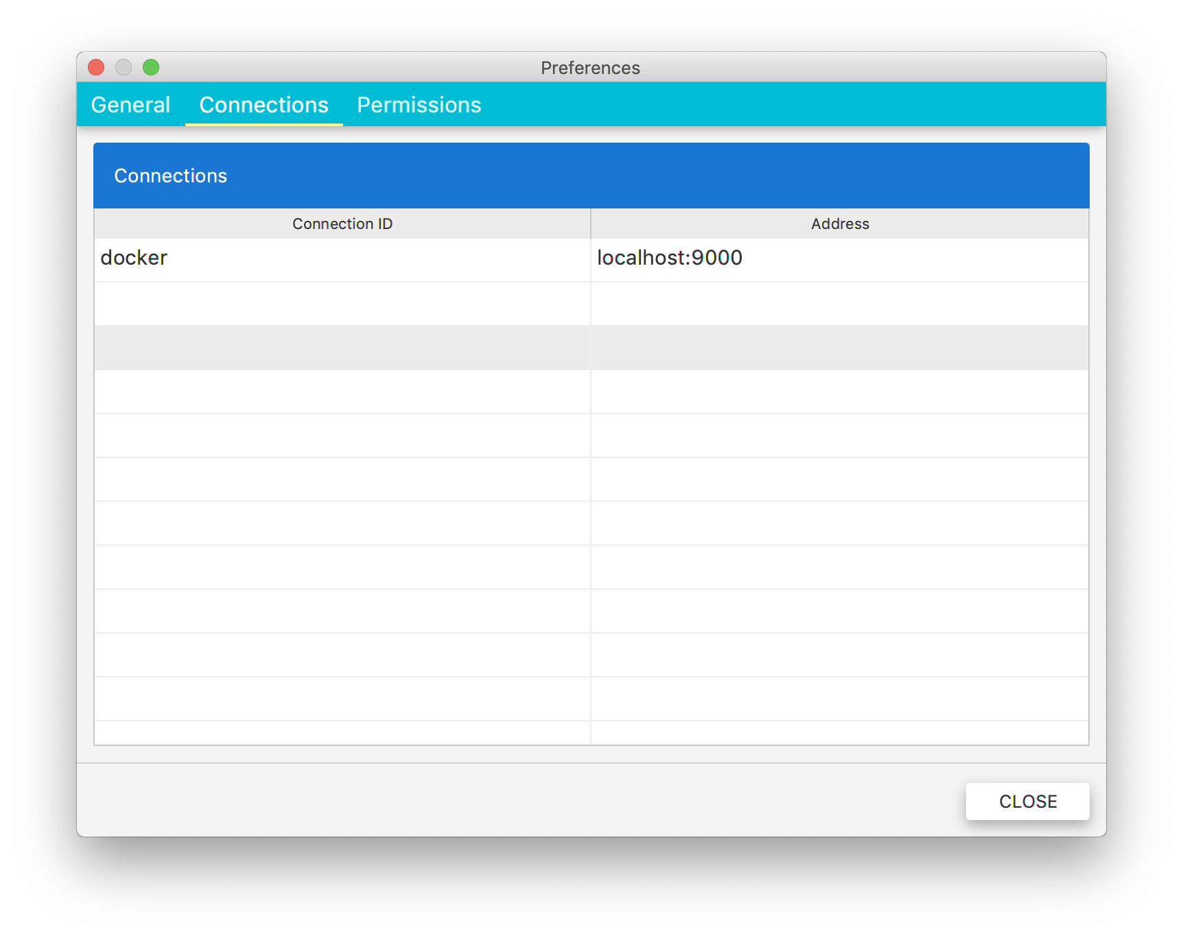
Fig. 4.3 Preferences: Connections
4.3. Permissions
In this view, you can check which permissions you are granted. These settings are read-only and can be changed only in manager (see Authorization for more details).

Fig. 4.4 Preferences: Permissions
5. Configurations
Agents configurations are managed from workstation. You must click the CONFIGURATIONS menu item in Fig. 3.5 view to get the list of all the configurations.
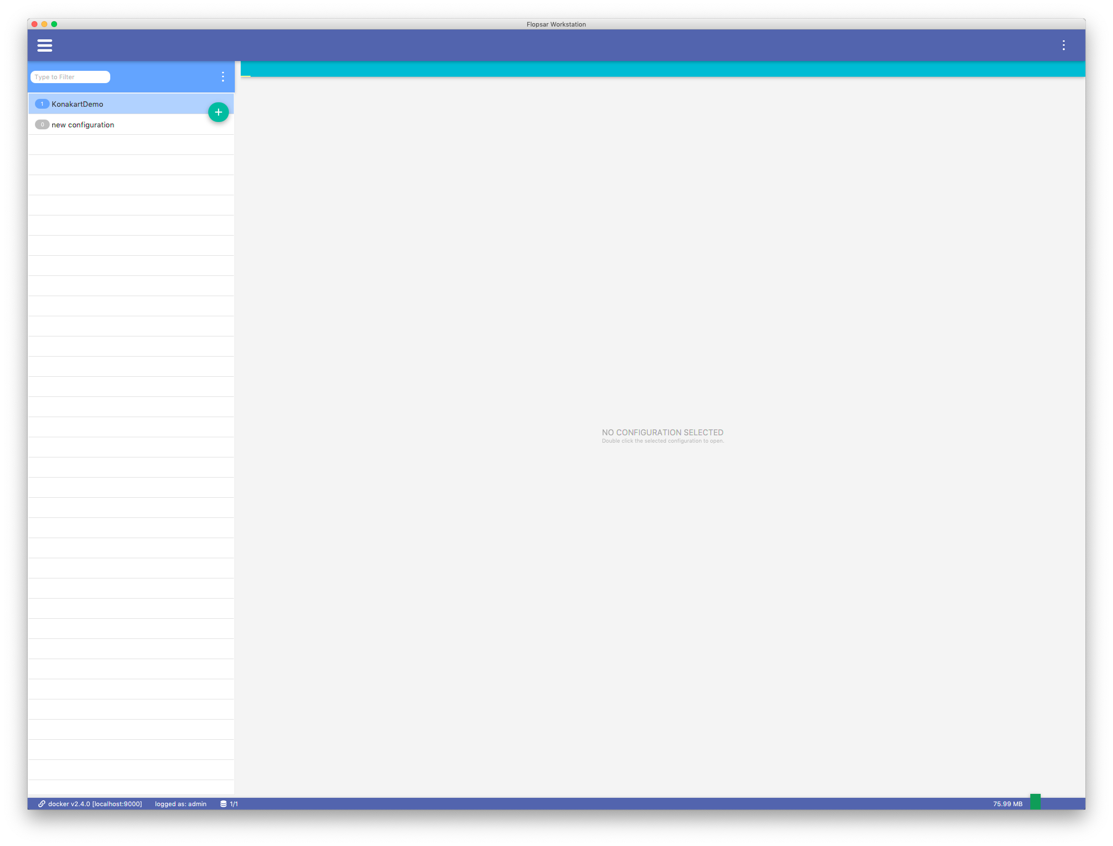
Fig. 5.7 Agents’ Configurations
Configurations are stored in the manager. When you double-click a selected configuration, the configuration is retrieved from the manager and displayed. Each configuration can have two copies: the active Fig. 5.9 and inactive Fig. 5.8 one. The active configuration is the one that is currently deployed. The inactive configuration is the one that is currently edited. If a configuration have both copies, the inactive one will be shown by default. You can switch between configurations using the edit icon, just before the configuration label.
In order to add a new configuration, click the + button.
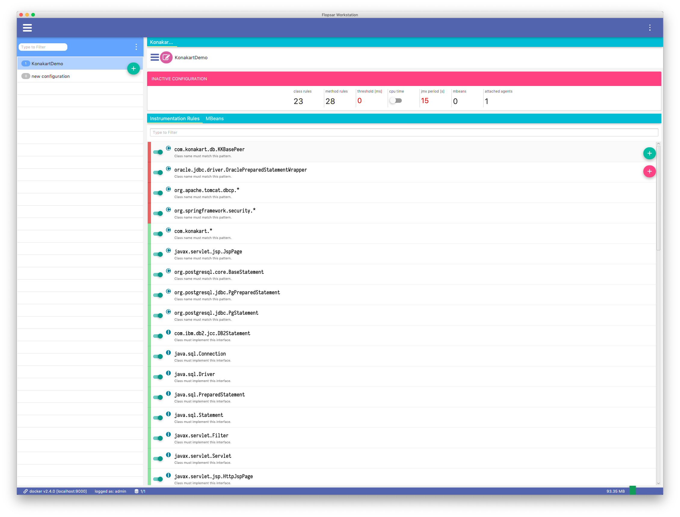
Fig. 5.8 Inactive Configuration
The edit view Fig. 5.8 is divided into two parts. The first tab is where you define instrumentation rules and the second one is where you define JMX beans to collect data from.
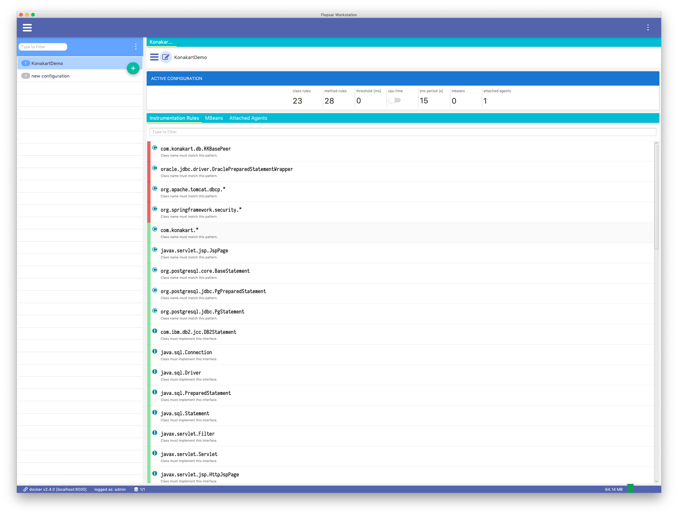
Fig. 5.9 Active Configuration
There is a third tab called Attached Agents in the active configuration view. You can select and attach/detach agents to the configuration in this tab.
5.1. Instrumentation Rules
Each instrumentation rule is either enabled or disabled. You can turn on and off rules using their toggle buttons. When a rule is disabled, it is not evaluated by agents.
There is either red or green bar at the beginning of each instrumentation rules entry. Exclusion rules are red and inclusion rules are green.
There are two + buttons in the list of instrumentation rules Fig. 5.8. If you want to define an inclusion rule you should click the green button, otherwise click the red one.
In the threshold field you can specify a threshold value for methods duration. In other words, you specify the lowest value of instrumented methods execution time above which these method calls will be reported. In the cpu time field you can select whether you want agents to report CPU time or not.
You have two types of rules at your disposal: exclusions and inclusions and two levels of rules: class and method ones. Basically, you should specify at least one inclusion rule for classes and one for methods to have a valid configuration.
Including Classes
In order to add a class level rule, select Class Rule from the green button menu. In the Fig. 5.10 form you specify which classes you want to instrument. If you want to match classes by their names, you should select the Class name radio button. If you want to instrument classes, which extend some super class, you should select the Super class. In this case you need to specify the fully qualified super class name. If you want to instrument classes which implement some interface, you should select the Interface. You must then specify a fully qualified name of the interface. Finally, if you want to instrument classes, which are annotated by some annotation, you should select the Annotation. You must then specify a fully qualified name of the annotation.
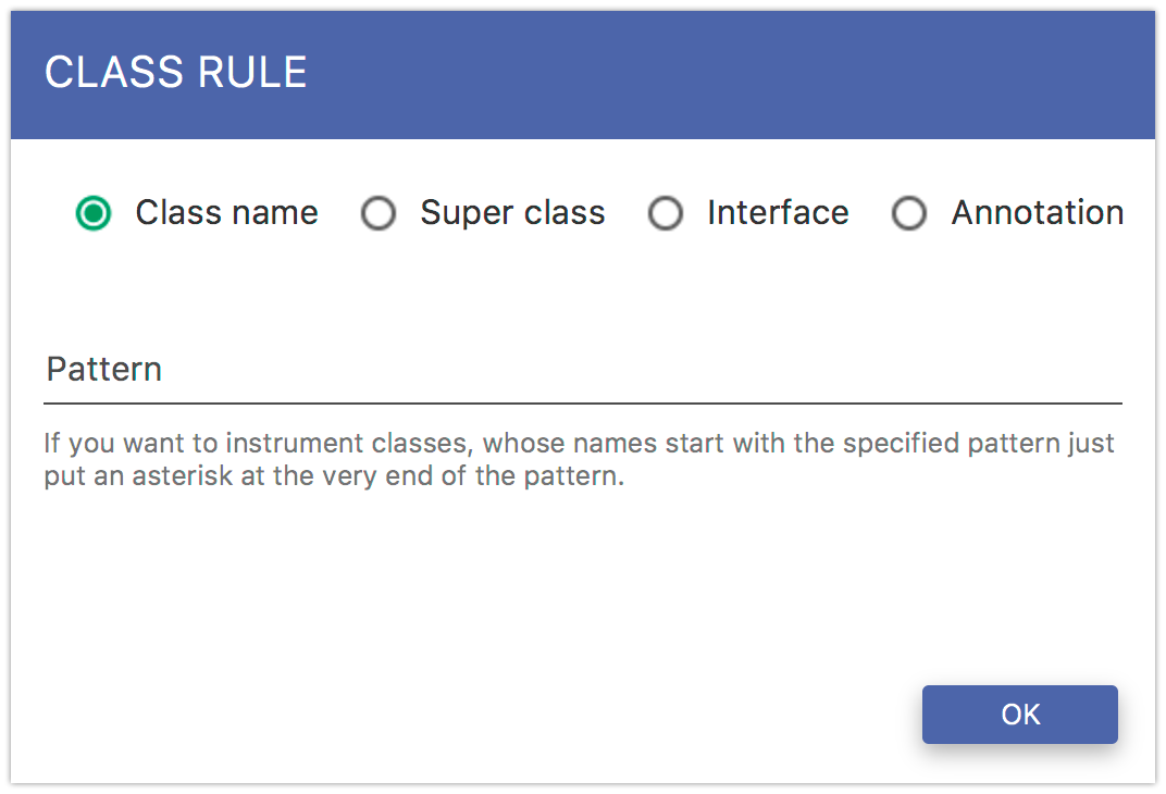
Fig. 5.10 Include Class Rule
If you want to instrument classes from particular packages, just select the Class from Packages from the green button menu. This operation will retrieve available packages from all the attached agents. You can add rules by double-clicking selected packages.
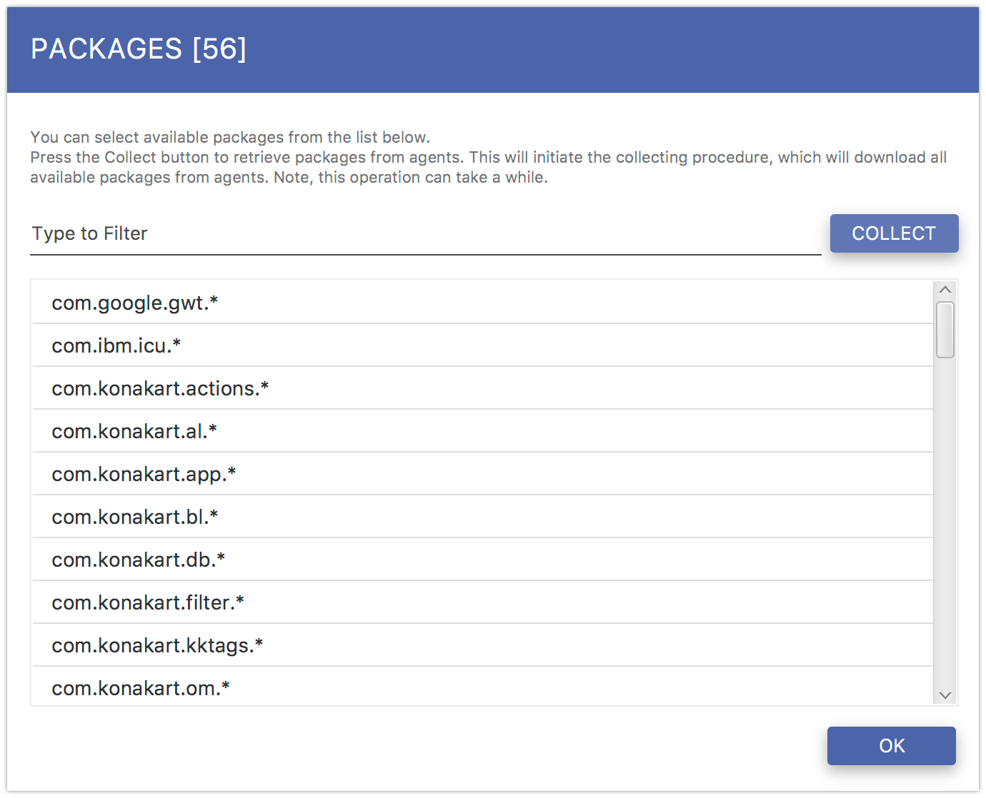
Fig. 5.11 Include Packages
Including Methods
In order to add a method level rule, select Method Rule from the green button menu. You can specify methods for instrumentation by their access modifiers. Just select the modifier so that those methods are instrumented, whose modifiers match one of the selected. You can also specify methods by exceptions they throw. Just select the Exception radio button and specify the exception class.
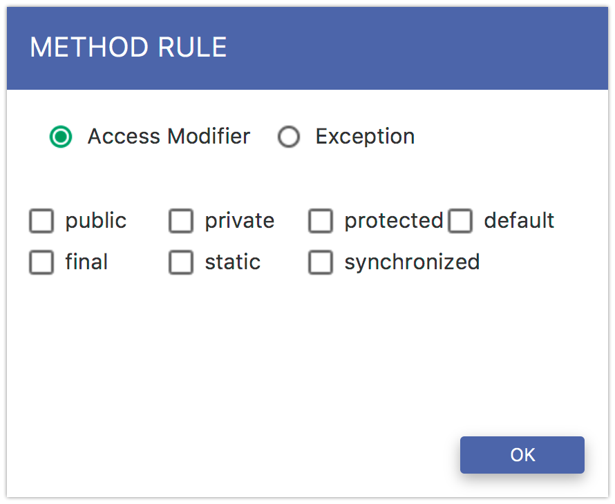
Fig. 5.12 Include Method Rule
If you want to instrument methods with formatters, you should select the Formatted Method Rule from the green button menu.
There are some input fields that need to be filled (Fig. 5.13). In the Class field you can specify the exact class, your instrumented method should belong to. If you do not want to specify the class, than you should select the Any checkbox.
Note
Please note that any method, which matches the specified pattern, in any class will be instrumented with the formatter if you select Any checkbox.
In the second field (text area), you must specify the exact method signature you want to instrument. You should ignore argument names and specify fully qualified class names of all objects. In the OPTIONS row you have three, additional options to select. If you want to ignore the configuration threshold, select the Ignore threshold checkbox. If you want to instrument the method on exit, select the Instrument on exit checkbox.
Now, if you want to report only parameter values without any preprocessing you can now click the OK button and you have your rule defined. However, if you want to add some custom processing you should select Custom formatter option.
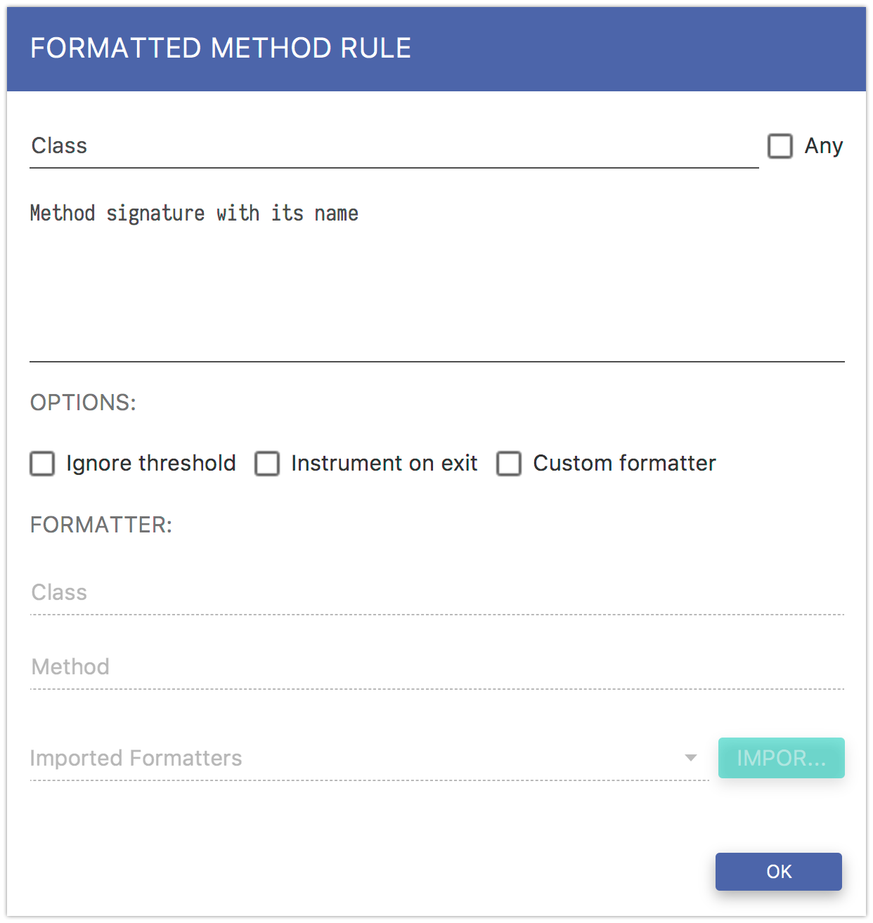
Fig. 5.13 Include Formatted Method Rule
First of all, you must then specify the formatter signature. There are two ways of specifying the formatter signature. The first one is to specify it manually by entering the class and the method name of your formatter. The second one is used when you already have some implemented formatters. You just need to click the IMPORT button and select a jar file with your formatters. The application will scan the jar and populate the formatters combo box with all the found and valid formatters. Select one of the formatters, click the OK button and you have your formatter rule created.
Excluding Classes
If you want to exclude some classes from the configuration, select the Class Rule from the red button menu. Then, specify the pattern for fully qualified class names. If you specify the asterisk at the end, the rule will match every class, whose fully qualified name starts with the specified pattern. Otherwise, the exact match will be checked.
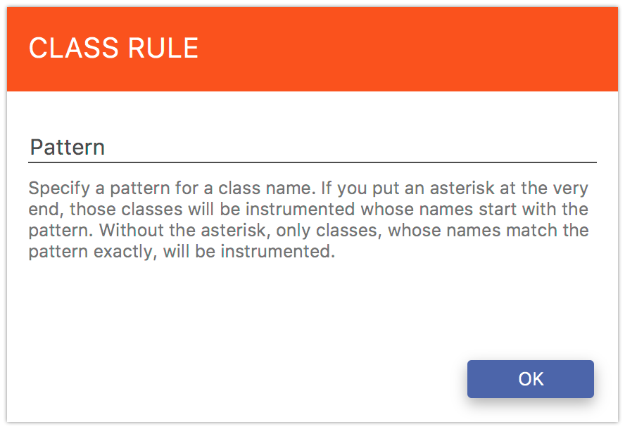
Fig. 5.14 Exclude Class
Excluding Methods
When you are done with classes rules, you need to specify some method rules. If you do not want to instrument getter/setter methods, you should select the Method Accessors from the red button menu.
Note
By setters/getters we mean accessor methods of a private instance field.
If you want to exclude some methods basing on their names, you should select the Method Rule from the red button menu. Here, you must specify a regular expression pattern for names. Finally, you can also exclude specific methods by selecting them from a list retrieved from running agents by selecting the Hot Methods tab (see Hot Methods for details).
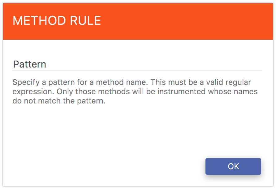
Fig. 5.15 Exclude Methods
5.2. Hot Methods
This feature enables you to record instrumented methods executions. The Hot methods feature is very useful, when you tune your configuration for minimal performance impact. In this way, you can easily detect the most frequently executed methods and exclude them from instrumentation, unless you really need to instrument them. You can also exclude classes using this feature.
You can use this feature only when you have some agents attached to your configuration. In other words, agents are able to report their hot methods if and only if they instrumented these methods earlier. That means, you cannot use this feature when you create a new configuration and the configuration has not been deployed yet. You must first deploy the configuration, attach some agents to it and then edit the configuration again. Only then, this feature will be available to you.
If you cannot see any entries in the table, click the Collect button in the bottom-left corner. This will trigger an operation of retrieving hot methods from all the attached agents.
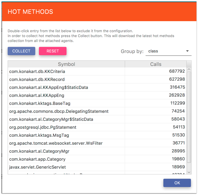
Fig. 5.16 Hot Methods
All the retrieved methods will populate the table Fig. 5.16. The results are always grouped by classes, methods, classes & methods or agents. You can exclude classes or methods only from views grouped by either emph{classes} or emph{methods} respectively. Views grouped by emph{classes & methods} and emph{agents} are only for information purposes. In order to exclude some entries, use a context menu over the table.
You can reset the results anytime and start to collect new results by clicking the Reset button. This will clear all the previous results and re-enable the Hot Methods feature on all the attached agents.
5.3. JMX
Configuring JMX for agents relies on specifying ObjectName patterns and the data collecting frequency. In the Period field you can specify how frequently agents must report data. In order to add some patterns, you must click the Manage MBeans menu.
Note
In order to add new ObjectName patterns, you must have some configuration deployed and some agents attached.
Adding new patterns requires you to deploy some configuration and attach some agents in the first place. MBeans can be imported only from running agents, so there must be some agents attached to the configuration. Assuming your setup fullfills the aforementioned conditions, click the Import MBeans… menu item. You should get a pop-up window with a list of available ObjectNames Fig. 5.17.
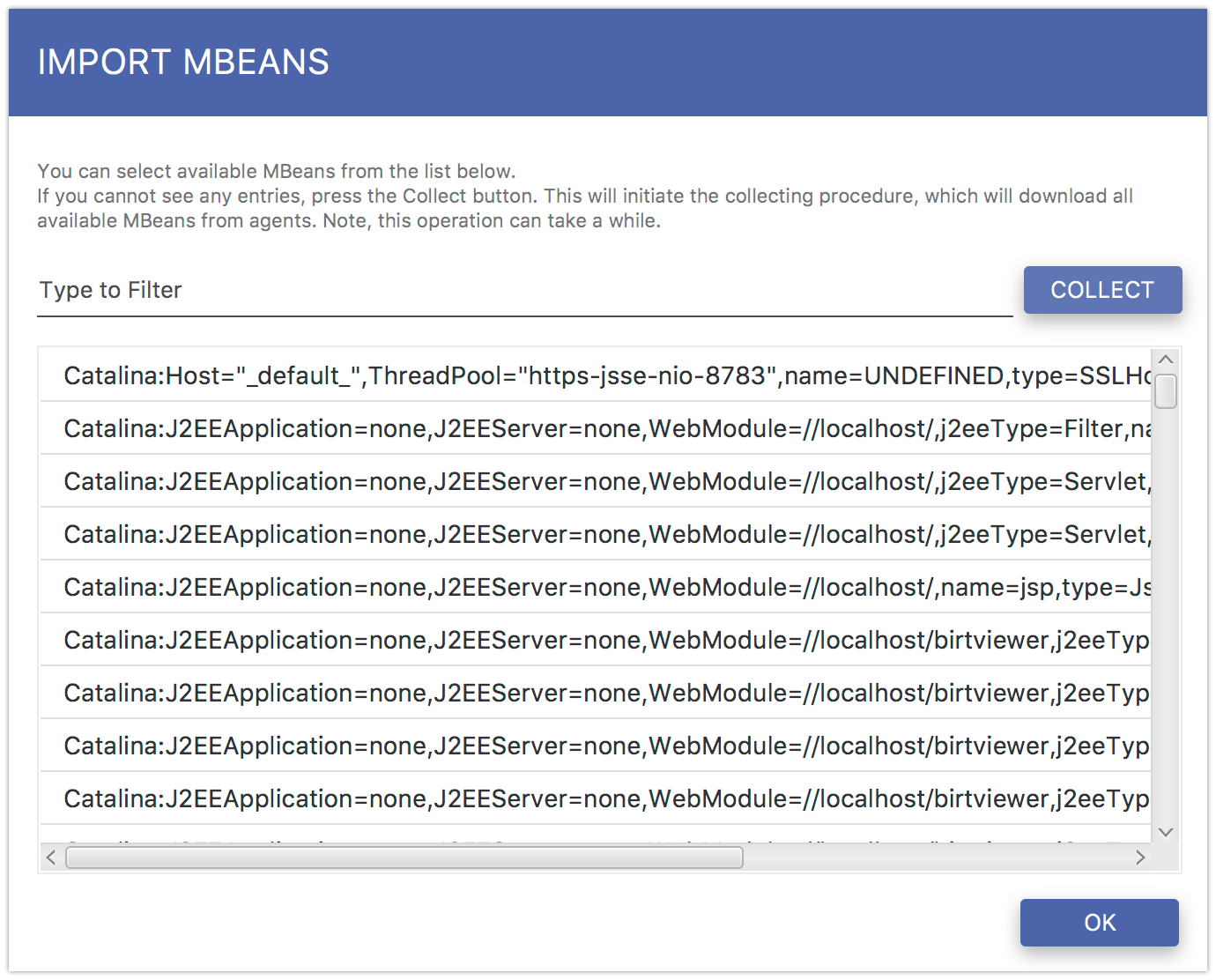
Fig. 5.17 Importing JMX ObjectNames
If the list is empty, click the Collect button in the bottom-left corner. This operation will collect all the available ObjectNames from all the attached agents. In order to add some selected record, either double-click the record or use the list context menu. When you are done with importing ObjectNames, click the Close button. Now, you should have the selected records added to the MBeans list in the Fig. 5.8 view.
Usually, most of ObjectNames is specific to the servers they come from. Their names contain a server specific data such as IP addresses, ports etc. That means there are ObjectNames that are available only on particular servers. In order to make them available on most of the servers and simplify the configuration we need to modify their ObjectNames. This can be achieved by clicking the Transform to Pattern… menu item in the list context menu. As a result you should get a similar pop-up window to this one Fig. 5.18.
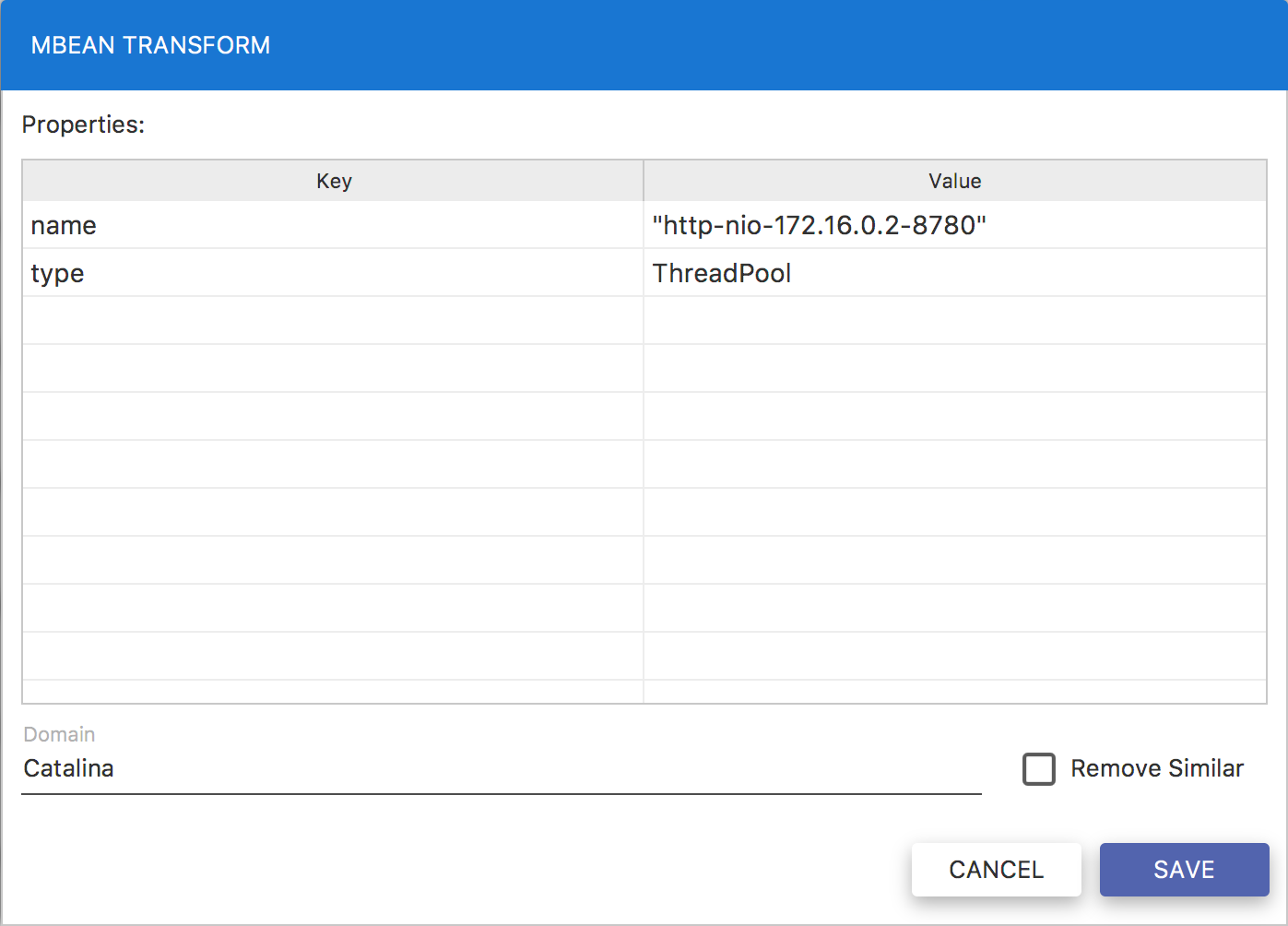
Fig. 5.18 Transforming ObjectName
This is a view of a decomposed ObjectName into keys and values. The Value column is editable so that you can replace values with custom ones and transform some specific ObjectName into a pattern. In order to edit the values just double-click the record and modify it. The Remove similar checkbox is used if you want to get rid of other, similar ObjectNames, whose name matches your pattern.
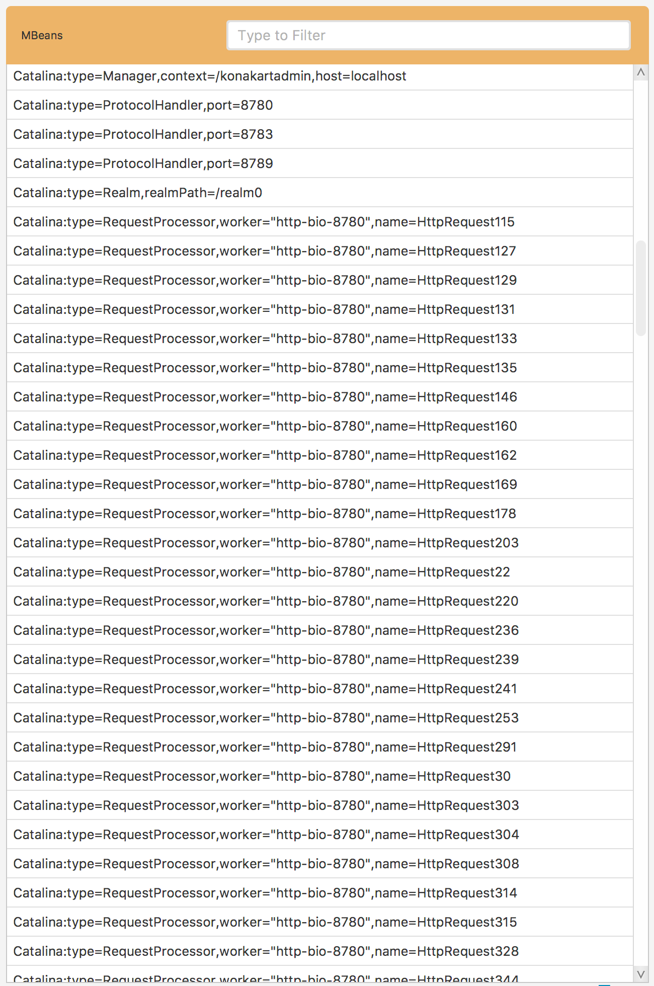
Fig. 5.19 Before Transformation
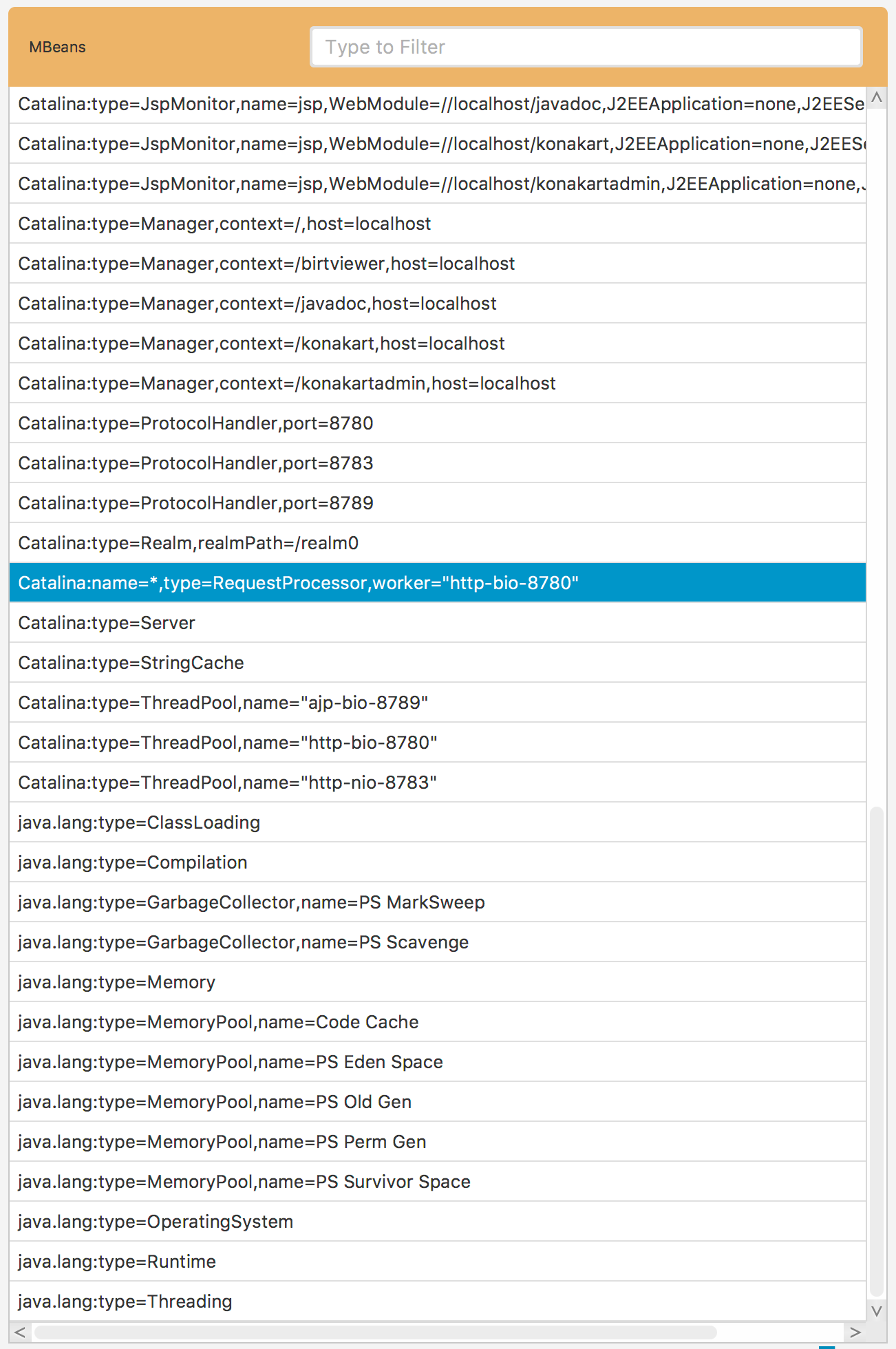
Fig. 5.20 After Transformation
In order to illustrate the transformation procedure see Fig. 5.19. There are multiple ObjectNames, which are very similar and the only key they differ is the name. By transforming the name value to * of just one of these similar records, we can easily simplify the entire set of similar records into a single ObjectName. That is exactly how the transformation procedure works.
5.4. Deploying Configurations
When your configuration is ready to be deployed, you should first save it by clicking the Save button in Fig. 5.8. This operation will only persist the configuration in the manager.
Warning
If you do not save your configuration before you exit workstation, all the changes you made will be lost.
In order to activate the configuration, you must click the Deploy button. This operation will make the configuration active. When the configuration is active, you can attach agents to it by clicking + button in Fig. 5.9.
During deployment operation all the attached agents are notified about it and the configuration is uploaded to them. The agents will check whether there are any changes between their current configuration and the new one. If the agents detect instrumentation rules changes, they will reload their configuration. The reloading operation duration can vary and it strongly depends on the configuration and application itself. It can take from a few seconds to a minute.
Warning
Configuration reloading is a heavy operation and will degrade your application performance temporarily. It can even halt the entire application for the time of reloading operation. Do not reload a configuration when your application is under heavy load.
6. Galaxies
Galaxies are special views of collected data. Basically, this is an alternative view of stacks executions, where stacks are represented as dots. You can access the galaxy view by clicking the GALAXIES menu item in the Fig. 3.5 view.
The galaxy is used to monitor recent 15 minutes of selected agent instances. They can be managed from the galaxy explorer Fig. 6.1.
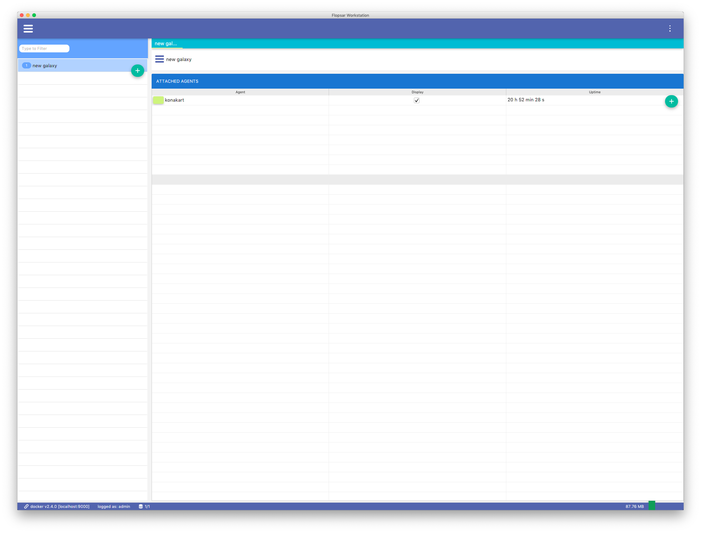
Fig. 6.1 Galaxies Explorer
A new galaxy can be added by double-clicking the + button. You can see the galaxy details by double-clicking the corresponding galaxy entry in the list on the left.
This view contains a table with three columns. There is an agent name along with a small, colored square in the first column. The color of the square is used to distinguish among various agents on the galaxy view. If you want to change the color, just click the square. The second column is editable and allows you to decide whether you want the agent to be displayed on the galaxy view. The third column shows the current uptime of the agent. If you want to open the galaxy view Fig. 6.2, just click the Show button.
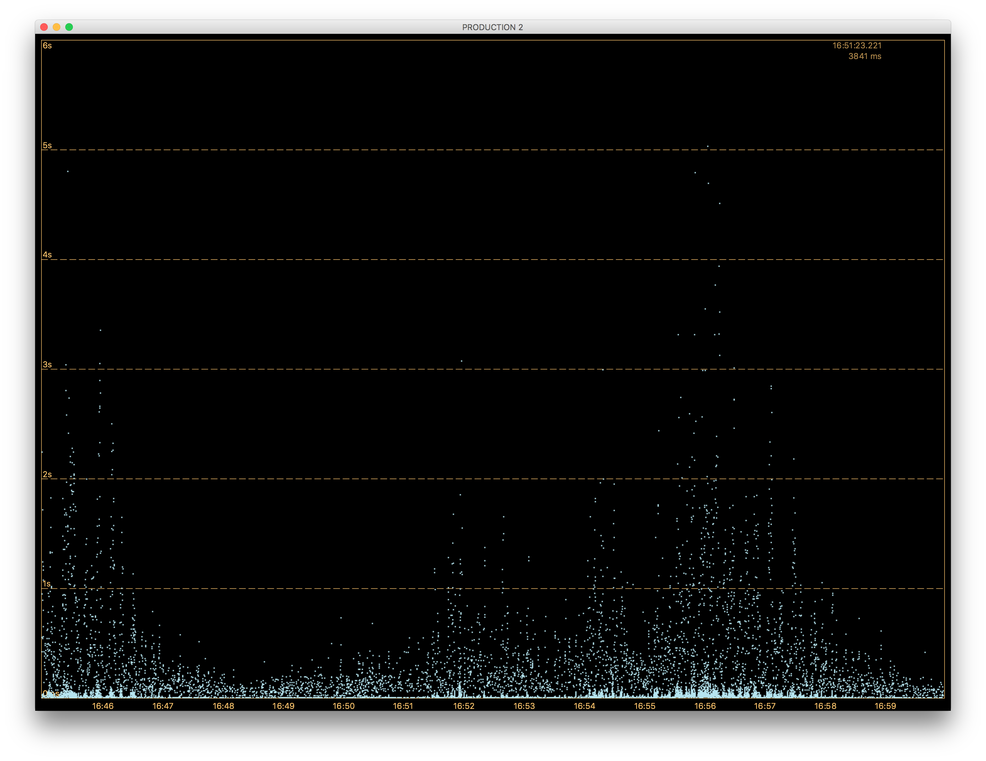
Fig. 6.2 Galaxy View
This is a live view of your attached agents. Each dot represents a single method execution. The method duration is displayed on the vertical axis. The horizontal axis shows a time axis and the whole view moves from right to the left as time goes by. If you want to change the graph scale, you can use your mouse scroll. In order to customize the graph, use its context menu Fig. 6.3.
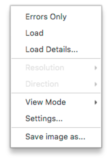
Fig. 6.3 Galaxy Context Menu
The context menu has several options, which enable you to customize your galaxy. It also provides auxiliary information about your data reported by the agents. If you want to see the total load of the attached agents, select the Load checkbox item. It will display a stacked area graph of the load for all the attached agents Fig. 6.4. The bottom area denotes those calls which threw exceptions. When the load is displayed, the number of total calls is displayed in the veritcal axis on the ride side of the graph.
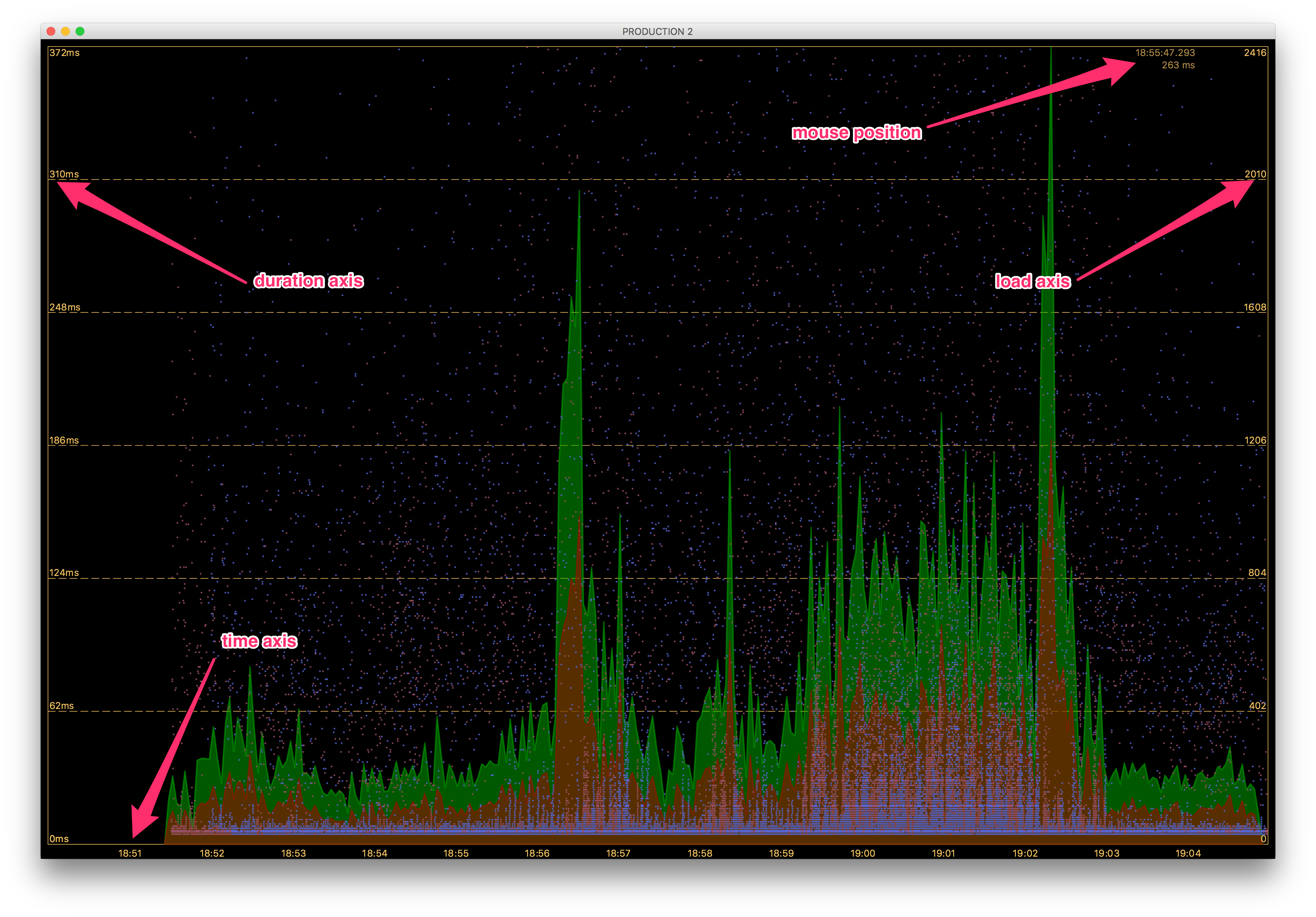
Fig. 6.4 Galaxy View: Load
This load view is an aggregated one so if you want to see how the load looks for each agent, click the Load details… menu item. You should see a view Fig. 6.5 with the table and the graph on it. The Errors column shows the total number of calls that threw exceptions. The Calls column shows the total number of calls.
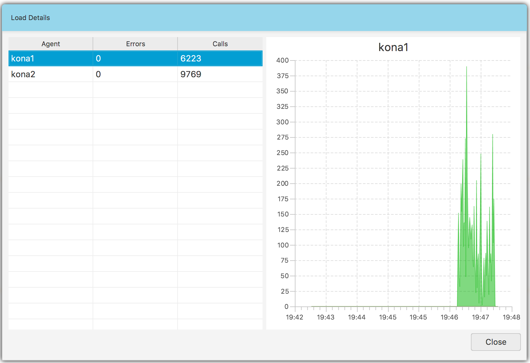
Fig. 6.5 Galaxy View: Load per Agent
If you want to customize some galaxy colors and scale, click the Settings… menu item. In the settings window Fig. 6.6 you can change background, selection, load backgrounds colors. You can also change the duration range on the vertical axis.
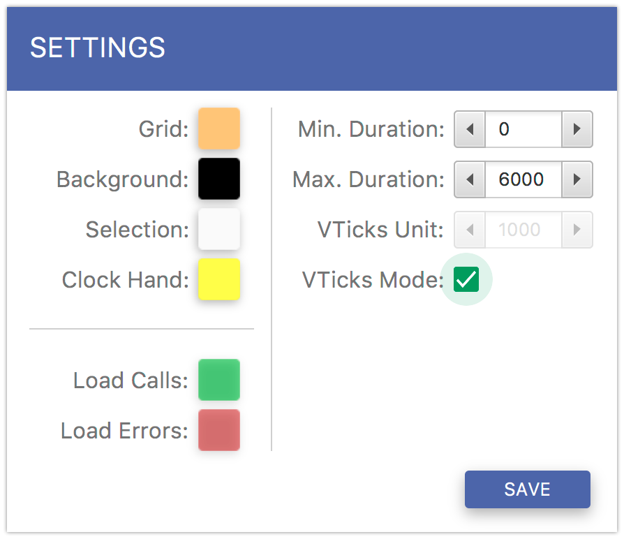
Fig. 6.6 Galaxy View Settings
Your can switch between two types of galaxies: flat and radar ones. If you want to switch to the radar Fig. 6.7, select the View Mode –> Radar menu item.
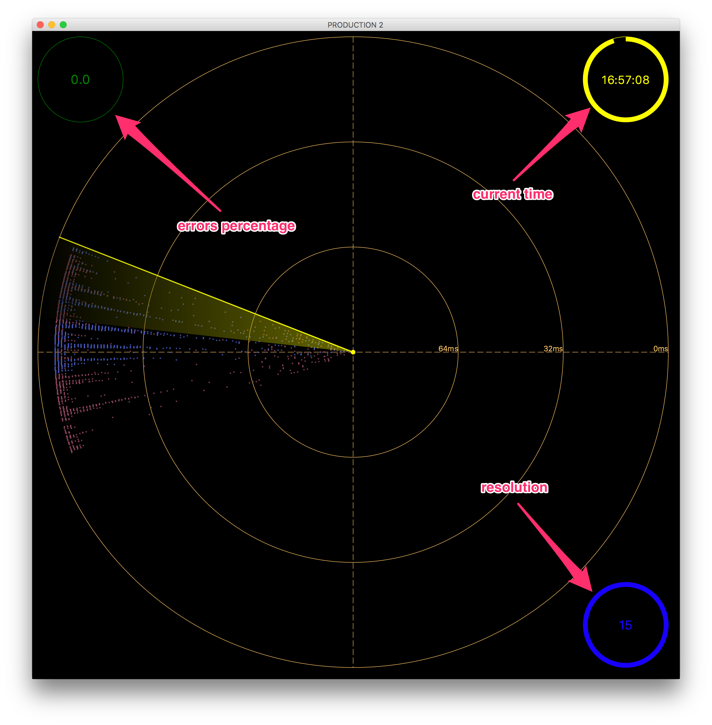
Fig. 6.7 Galaxy View: Radar
If you want to display only those method calls, which throw exception then select the Errors only checkbox item.
Galaxy Radar
7. Agents
Agents health can be viewed by double-clicking the AGENTS item in the side menu Fig. 3.5. If you click on some selected agent pane, you will see its status and health details.
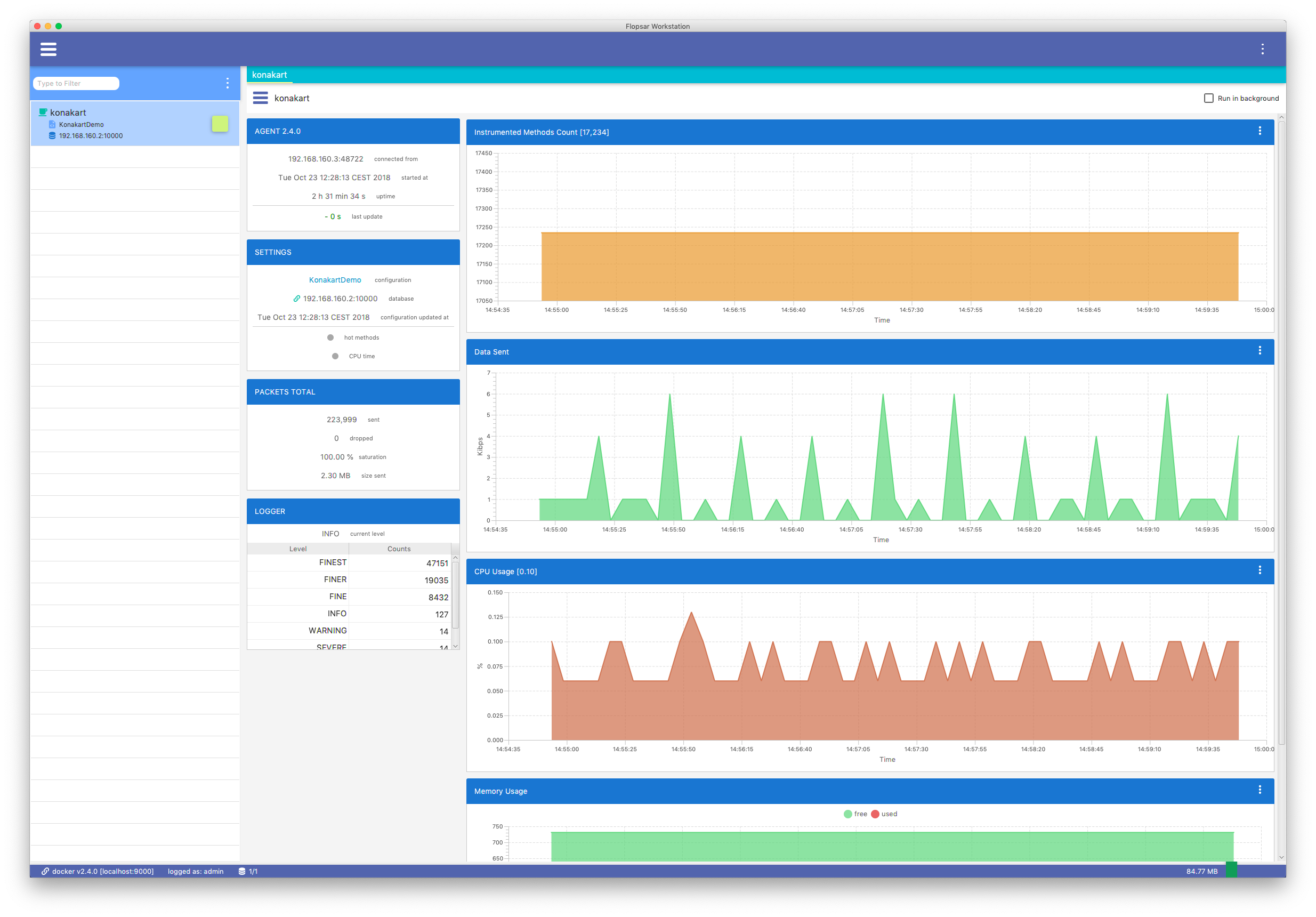
Fig. 7.1 Agent Status View
The view is divided into panes with either text information or graph on them. All the information in this view is reported by the agent. The reported data are collected from the agent start and reset everytime the agent restarts.
The AGENT pane contains the following data:
| connected from: | Source socket address of the agent. It shows from which socket address the agent connects to manager. |
|---|---|
| started at: | Agent startup time. It shows when the agent started. |
| uptime: | Agent uptime time. It shows how long the agent is up. |
| last update: | Agent last report time. It shows how much time has passed since the last agent report received by workstation. When this time is greater than 15 seconds, its color turns from green to red. |
The SETTINGS pane contains the following data:
| configuration: | Current configuration. It shows the configuration the agent is attached to. |
|---|---|
| database: | Current database. It shows the database the agent sends its data to. |
| configuration updated at: | |
| Agent configuration deployment time. It shows the last time a configuration has been deployed to the agent. | |
| hot methods: | Hot Methods feature. It shows whether the Hot Methods feature is enabled or disabled. |
| CPU time: | CPU time feature. It shows whether the CPU time measurement is enabled or disabled. |
The PACKETS TOTAL pane contains the following data:
| sent: | Number of sent packets. Each method call, symbol or some metric value is represented as a single packet. These packets are sent to a database. This shows the total number of such packets sent to the database from the moment of the agent start. If the agent is attached to another database, this value will be reset. |
|---|---|
| dropped: | Number of dropped packets. It shows the number of packets that have been dropped inside the agents. There can be a few reasons which make the agent to drop packets. See Data Collecting Considerations for details. |
| saturation: | Packets saturation. It shows the ratio of the number of received packets to the total number of packets. This total number is a sum of dropped and received packets. The value is displayed in percentages. If the value is 100% it means that all the packets, that have been collected on the agent, have been received by the database. If this value is low, it means that a large number of packets is dropped for some reason. |
| size sent: | Data size sent. It shows how much data has been sent to the database. This value is counted from the moment of the agent start. If the agent is attached to another database, this value will be reset. |
The LOGGER pane contains the following data:
| current level: | Logger level. It shows the current logger level set. |
|---|---|
| table: | Number of messages logged at the corresponding logger level. |
7.1. Charts
There are five charts presenting additional information. You can change the order they appear. The following charts are presented in order of the default appearance:
- This graph presents how many methods are currently instrumented.
- This graph presents how much data is sent from the agent. The unit is Kibps (1024 bits per second).
- This graph shows the CPU usage of the monitored Java process. Please note, this feature is available only for GNU/Linux machines.
- This graph presents the memory usage of the Java process.
7.2. System Properties
If you want to retrieve JVM system properties, just select the System Properties menu item in Fig. 7.1.
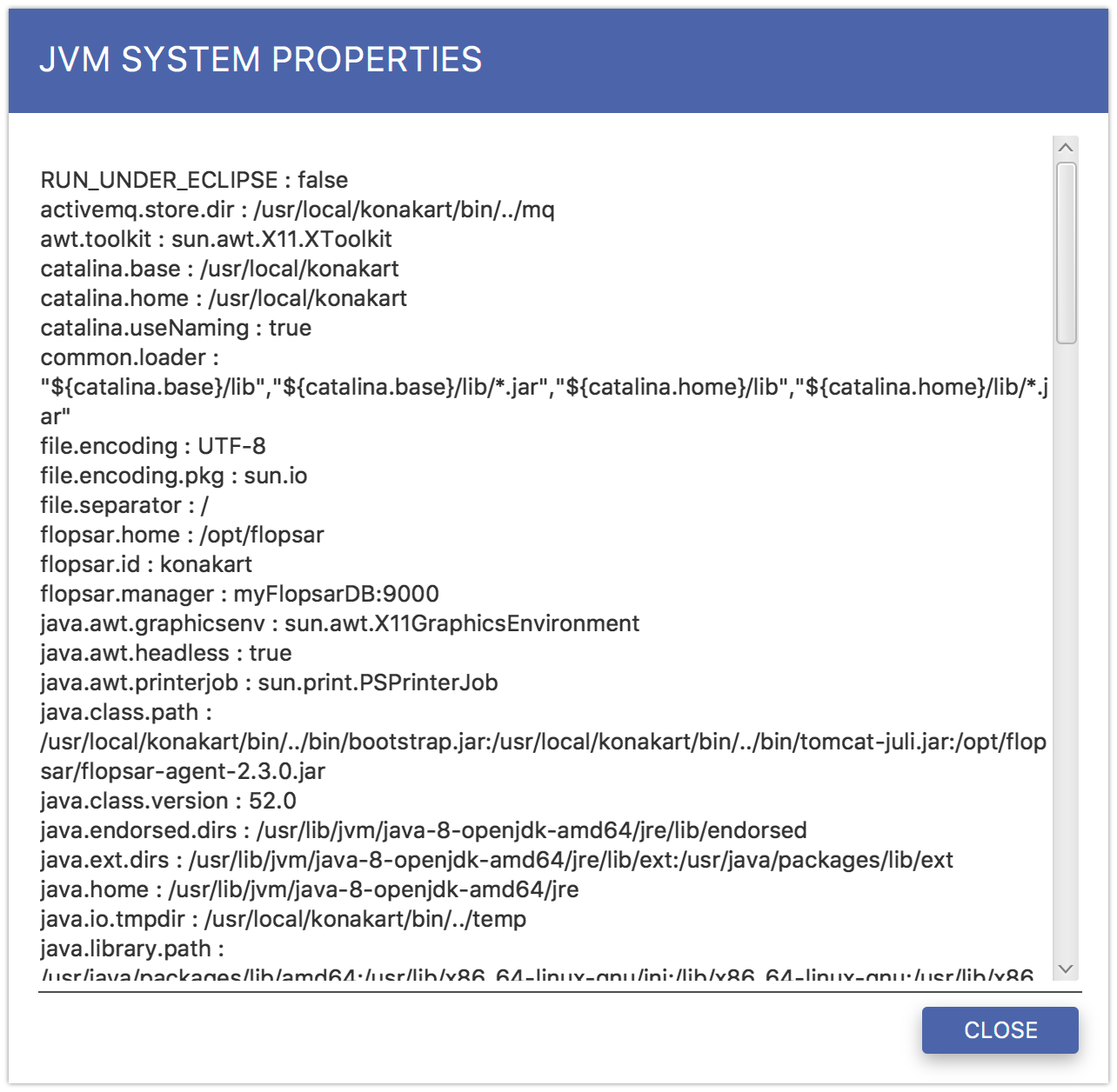
Fig. 7.2 JVM System Properties
7.3. Application Packages
This feature is useful if you want to know what packages are available in your Java environment, so that you can add some class rules to your configuration. The packages are reported up to the third level.

Fig. 7.3 Available Packages
7.4. Class Loaders
You can retrieve a list of classloaders detected by the agent. The result is presented in the form of a table. Each reported class loader can be in one of the four available states:
| PENDING: | to be instrumented, |
|---|---|
| NO NEED: | has been checked and no instrumentation is needed, |
| SKIPPED: | has not been checked and will not be instrumented, |
| INSTRUM: | has been instrumented. |
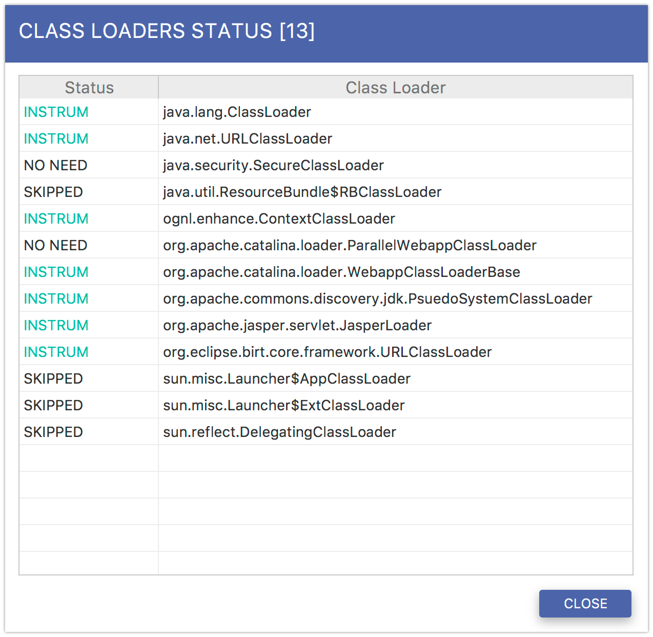
Fig. 7.4 Class Loaders report
8. Queries
Whenever a query requires you to specify a time range, you must fill out the form below.
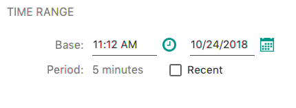
Fig. 8.1 Time Range Form
You have two time range types to choose from. If you want to define an arbitrary period of time, you must specify both the base time and its range. The resulting time range will span from the base time minus half of the specified range to the base time plus half of the range. In order to specify the time range just click the value of the Period and select a value from the pop-up menu. If you want to define a recent time period, just select the Recent checkbox and specify the range.
In case a query requires you to specify an agents pattern, you must fill out the form below.
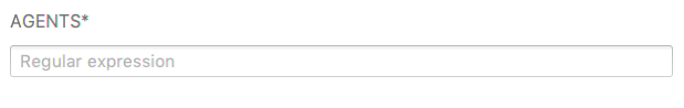
Fig. 8.2 Agents Form
The pattern entry must be a valid regular expression. The input field has an autocomplete feature, so if you want to select one of the available agents, just enter space and select from the pop-up list.
Any other entries depend on a selected query.
8.1. Flame Graph of Transactions
This query requires you to specify both a regular expression for agents and a time range.
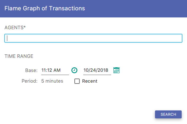
Fig. 8.3 Flame Graph Form
When you click the SEARCH button in Fig. 8.23, you will get a Flame Graph view Fig. 8.26. This view presents an aggregated form of the execution stack. It is composed of frames (rectangles), which represent aggregated methods executions. The y-axis presents the stack depth. Although the x-axis itself has no meaning, the width of frames has one. There are three criteria, that change the way you define the frames width. These criteria can be selected exclusively on the top pane by clicking one of the radio buttons: CALLS, CPU and OFF-CPU. When the CALLS is selected, the frames width denotes how often a particular method was executed within the stack.
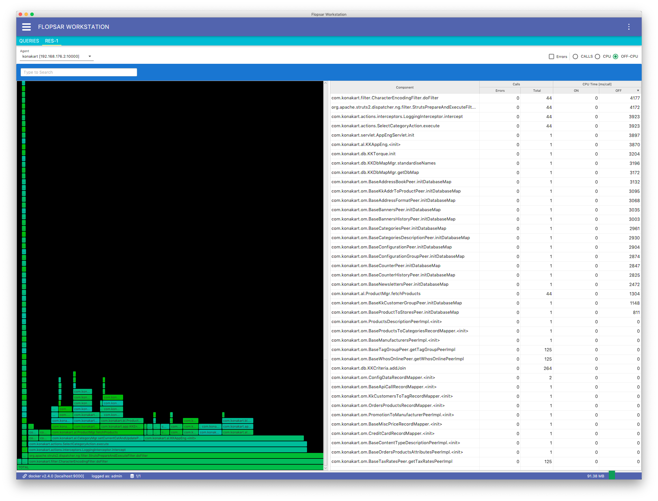
Fig. 8.4 Flame Graph
Note
Please, note there can be multiple frames representing the same method. This situation happens when a method is called in multiple places (on different execution levels) within the stack.
When the CPU is selected, the frames width shows how long methods spend on the CPU executing their code. Finally, when the OFF-CPU is selected, the frames width shows how long methods spend off the CPU.
The right side view of Fig. 8.4 presents a distribution of calls in the flame graph. Only a limited number of calls is displayed for both CPU and OFF-CPU sets. By right-clicking on a selected record, you get a single menu item Find on Flame Graph from the context menu. When you click the menu item, each corresponding frame will be highlighted. In this way you can easily find where your method is located in the Flame Graph.
Note
The Flame Graph visualizations were introduced by Brendan Gregg. For more details about flame graphs please refer to http://www.brendangregg.com/flamegraphs.html.
8.2. Galaxy of Transactions
This query allows you to explore data in a view similar to Galaxies. The query requires you to fill out the form below.
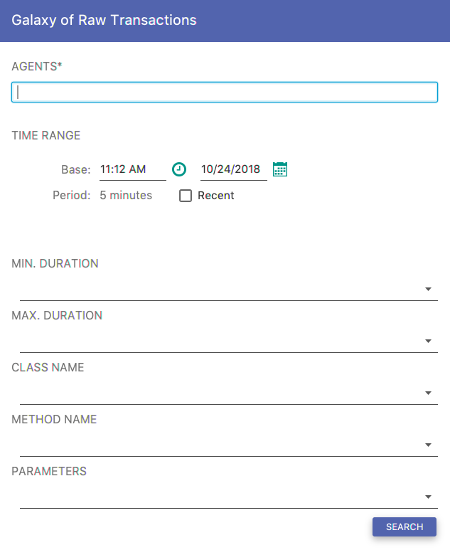
Fig. 8.5 Raw Transactions Form
When you click the Search button, you should get a similar result to Fig. 8.6. The view is divided into two regions. The left view presents your query results in a form of galaxy. The right view contains a table of those agents, whose data are displayed on the galaxy. In the first column, there is an agent name and its color. You can change this color by clicking the small square and selecting a new color. In the second column, you can either show or hide the data corresponding to the selected agent. The third column contains a total share of calls of the corresponding agent on the galaxy. The last column contains a total share of exceptions throws by calls of the corresponding agent. You can either show or hide this table by clicking on the toggle button Agents in the right-top corner of the view.
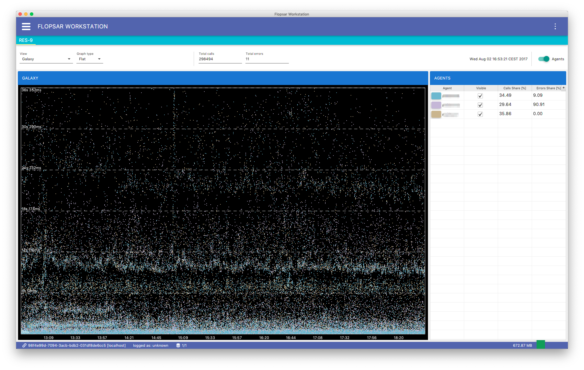
Fig. 8.6 Galaxy Result
The galaxy context menu Fig. 8.7 allows you to extend the analysis. If you select the Load menu item, you will get the load view in a form of a stacked area graph. The area colors correspond to the agents data. When the load is displayed, the calls count values are displayed on the right vertical axis.
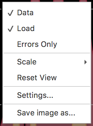
Fig. 8.7 Galaxy Result Context Menu
Using the Scale submenu you can change the graph scale which can be either linear or logarithmic. If you click the Settings menu item you can change the galaxy background and foreground colors.
If you want to find out what method calls are displayed, just click and drag your mouse to create a rectangle which covers the area you are interested in. If you release the mouse button, a pop-up menu will appear with two options. If you are interested in an exact list of transactions from the selected area, just select the Raw Transactions menu item. If you want to make a flame graph out of the selected transactions, select the Flame Graph menu item.
Besides, the galaxy flat view, your query results can be presented in a form of galaxy clock view Fig. 8.8. The view projects data onto a clock face. You can see only data from twelve hours range at a time. Use the AM, PM radio buttons and the date picker to change time.
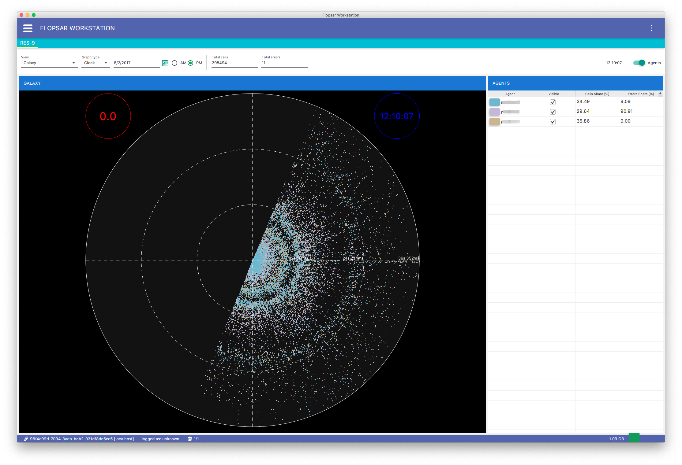
Fig. 8.8 Galaxy Clock View
Additionally, there are two extra views available. They can be displayed by clicking the Manage –> Switch View submenu and selecting one of the available items. If the Duration Distribution item is selected, Fig. 8.10 view will be displayed. If the Calls Distribution is selected, Fig. 8.9 view will be displayed.
Calls Distribution
This stacked-bar chart Fig. 8.9 presents methods calls distribution with respect to duration. Each color represents a single agent. The y-axis presents the number of calls. You can adjust both bar width (in milliseconds) and duration range (in milliseconds).
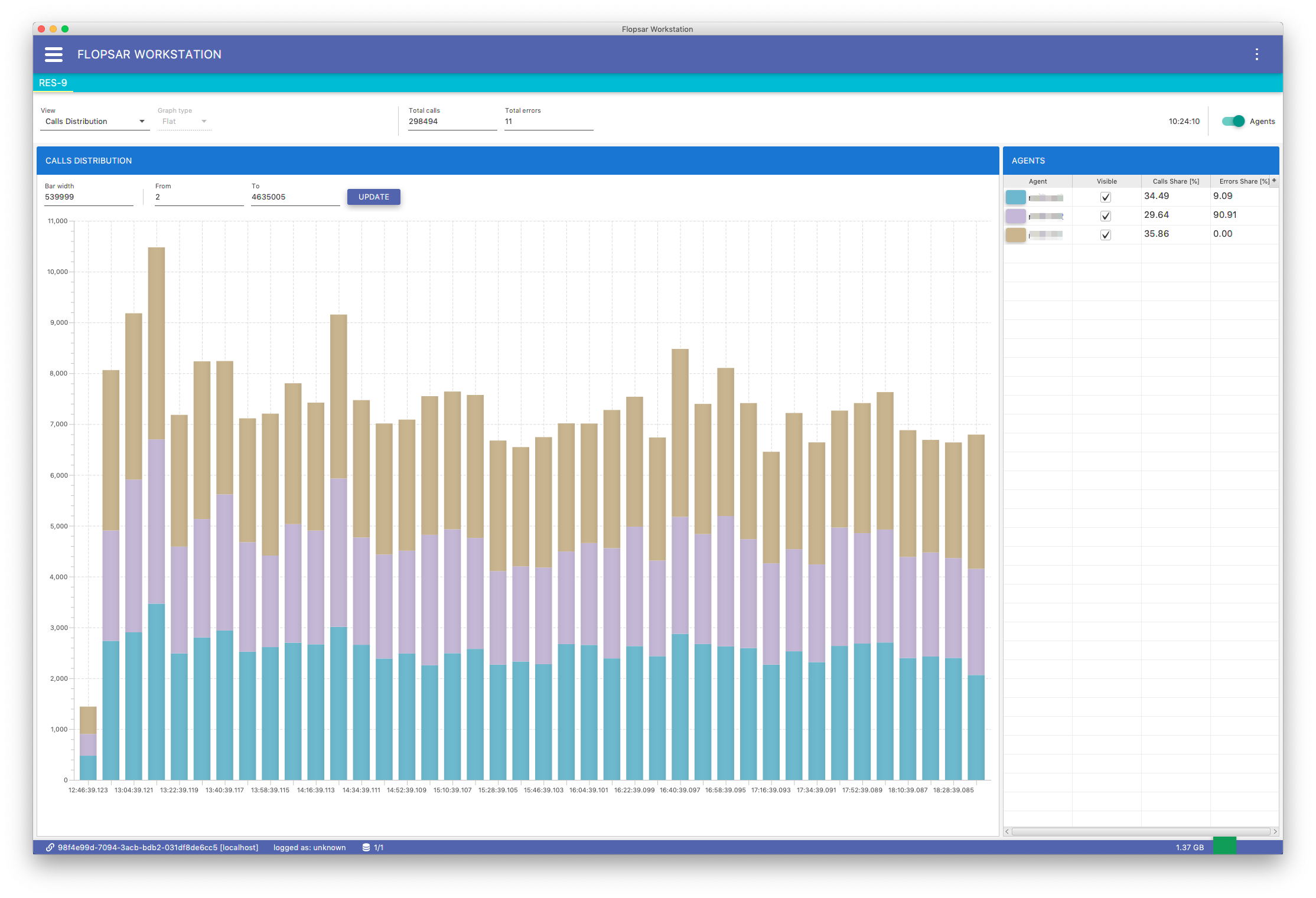
Fig. 8.9 Galaxy Calls Distribution
Duration Distribution
This stacked-bar chart Fig. 8.10 presents methods duration distribution with respect to time. Each color represents a single agent. The y-axis presents the number of calls. You can adjust both bar width (in milliseconds) and duration range (in milliseconds).
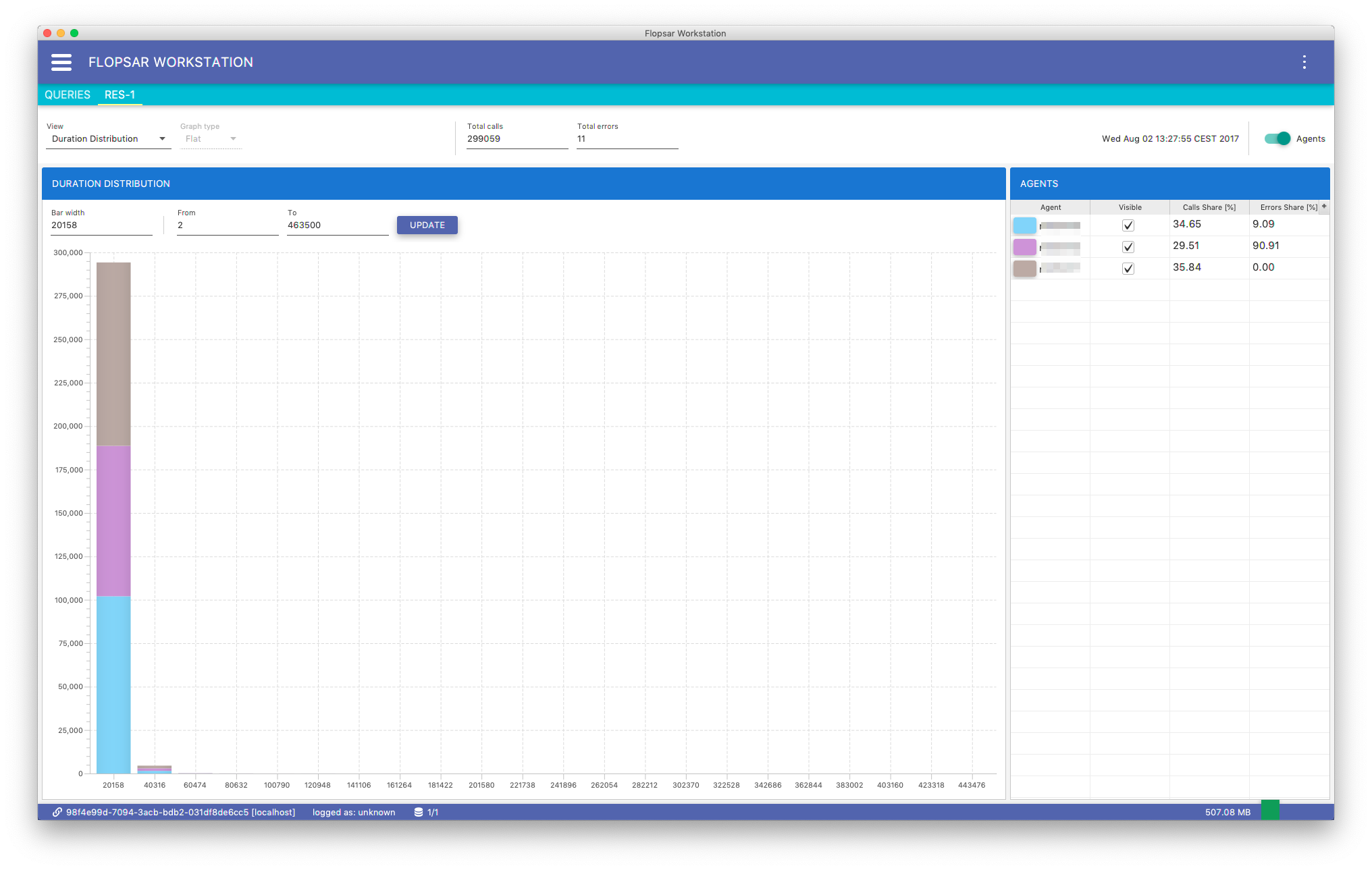
Fig. 8.10 Galaxy Duration Distribution
When you double-click in a bar in either Fig. 8.9 or Fig. 8.10, you will get a view Fig. 8.11, with list of methods from this bar.
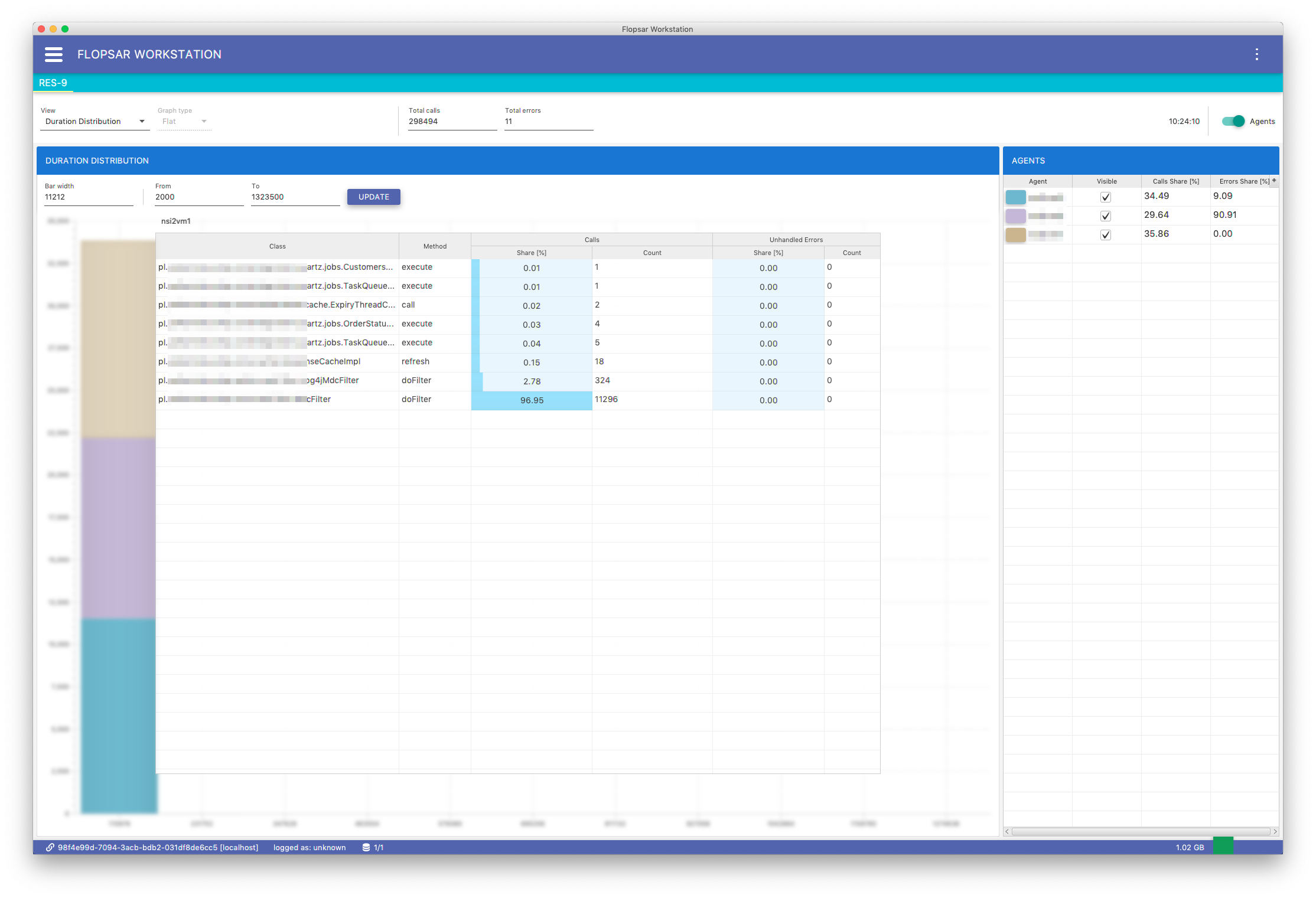
Fig. 8.11 Galaxy Duration Distribution: Bar Content
8.3. Garbage Collector
This query retrieves a list of garbage collector metrics for a specified agents pattern. When you click the SEARCH, you will get the list Fig. 8.13.
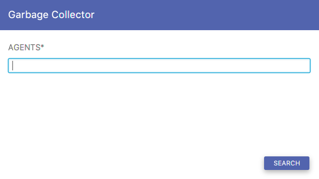
Fig. 8.12 Garbage Collector Form
You can select one of the available metrics from the list below and draw a graph for a specified time range.
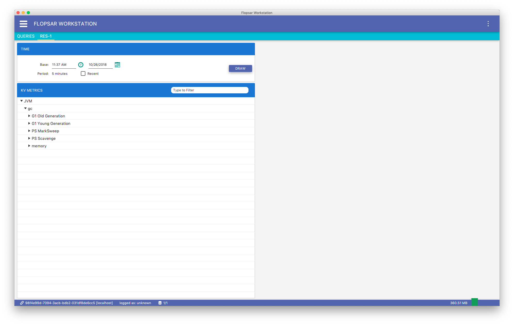
Fig. 8.13 Garbage Collectors
This is basically, the same view as in the Generic Key-Value Metric.
8.4. Generic Key-Value Metric
This query retrieves a list of all available metrics’ keys. The query requires you to specify a pattern for the key, which must be a valid regular expression.
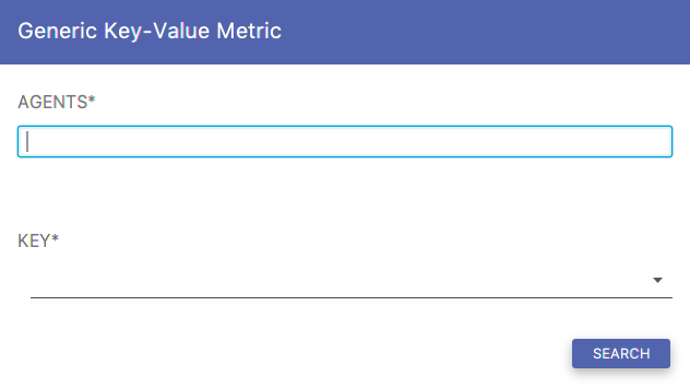
Fig. 8.14 Data Explorer: Environment Form
When you click the SEARCH button, you will get the output similar to Fig. 8.15. The view contains a tree with all the found metrics keys. Each tree leaf has a context menu, which enables you to make a quick graph for the last 15, 30, 60 or 120 minutes. If you want to specify an exact time range for a graph, use the time range form at the top of the view. If you either use quick graph or time range form, you should get a graph on the right side of the view. Each time you make a graph, it is added to the graphs list on the right. If you want to remove a graph from the list, just click the cross icon in the top-right corner of the selected graph.
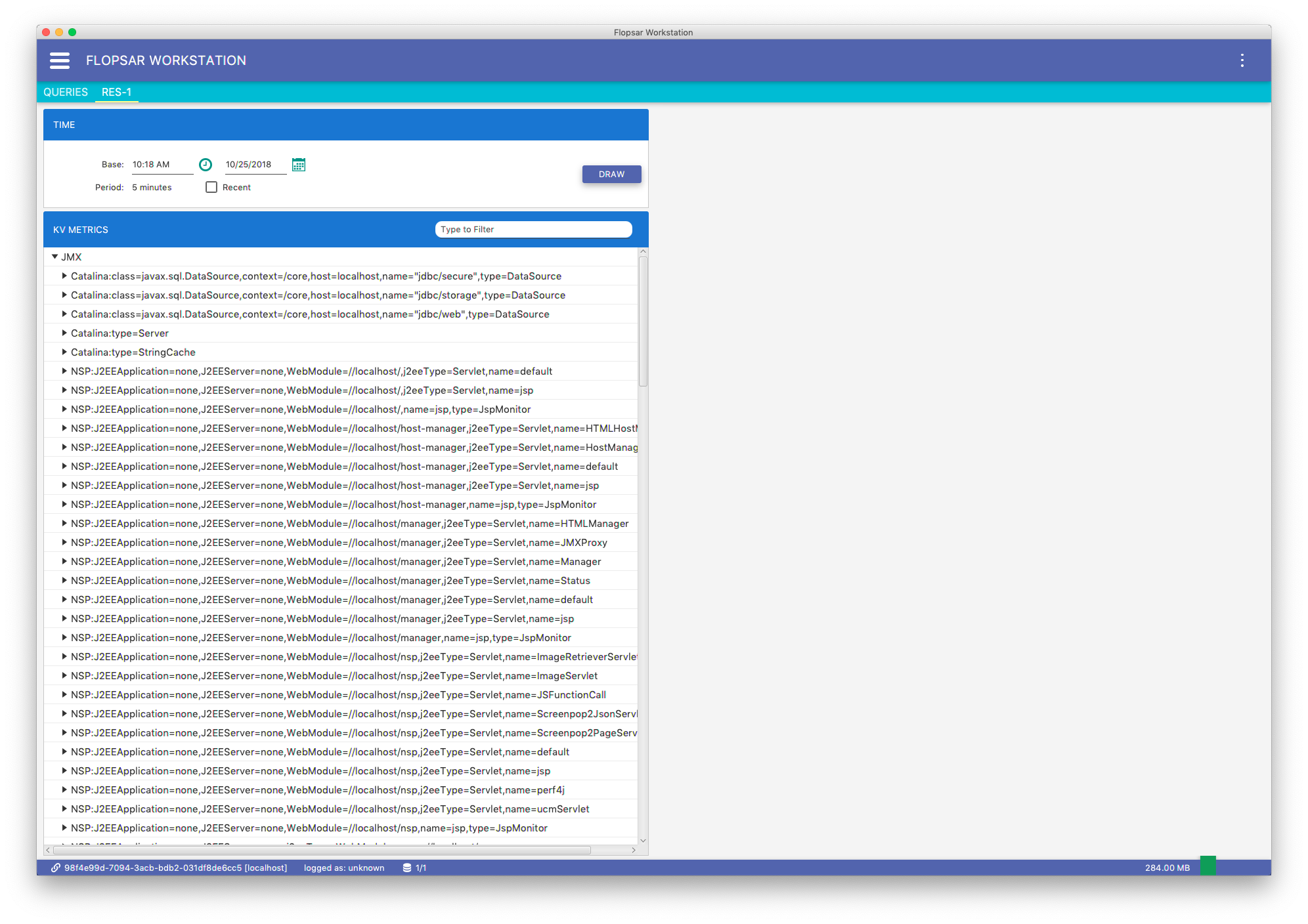
Fig. 8.15 Data Explorer: Environment Data Keys
When you click the DRAW button, the workstation sends a request to each database it is connected to and retrieves metrics for each agent, provided that the metric exists for the agent. As a result, there can be multiple graphs on a single graph pane and each graph corresponds to some agent. You can show or hide specific agents graphs by selecting the corresponding menu checkboxes from the context menu in the graph.
The graphs vertical axis displays raw values, in other words the values that are collected by agents. No unit is displayed because workstation knows nothing about the data it retrieves. It can be any data, provided by either agent or some user customized agent. In case of JMX data, please refer to your application documentation to find out what units your JMX metrics use.
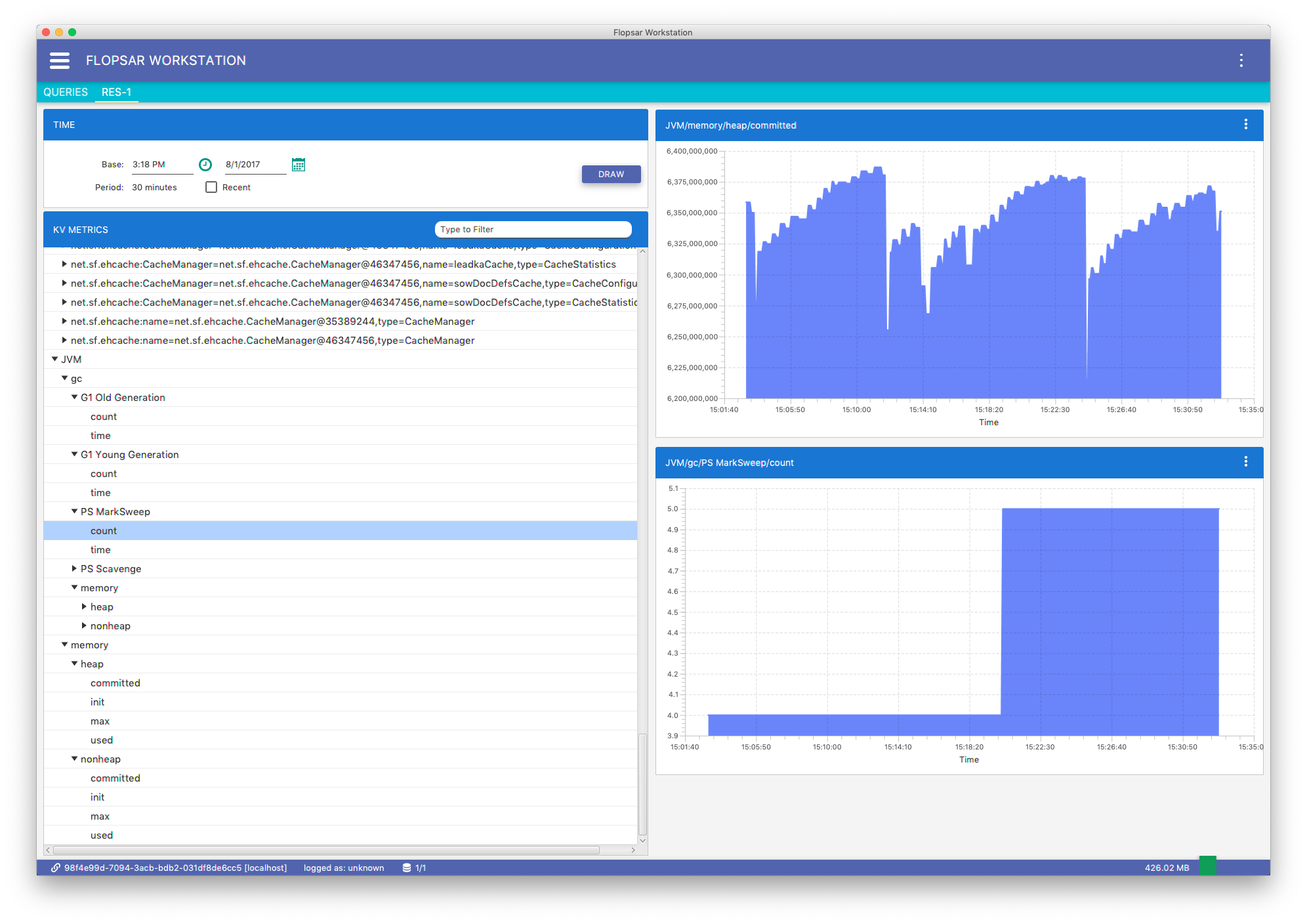
Fig. 8.16 Key-Value Data Graphs
8.5. Method Execution Analysis
This query retrieves an execution analysis of the specified method. The query requires you to specify both a class name and a method signature. The class name must be fully qualified Java class name and the method signature must be specified along with its name, for example void someMethod(int, long, java.lang.String). Optionally, you can specify a parameter key for the method along with a pattern for its value. The key entry must match one of the exisiting method keys and the value must be a valid regular expression.
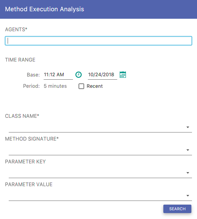
Fig. 8.17 Method Execution Analysis Form
Depending on the PARAMETER VALUE text field value you can obtain different results. If you do not use a subexpression (expression in parentheses), you will obtain the result similar to Fig. 8.19. If you use a subexpression, you will get the result similar to Fig. 8.18.
Note
Only a single subexpression in the PARAMETER VALUE text field is allowed.
In other words, if you want to obtain results grouped by some expression, you should put that expression pattern in parentheses so that it forms a subexpression.
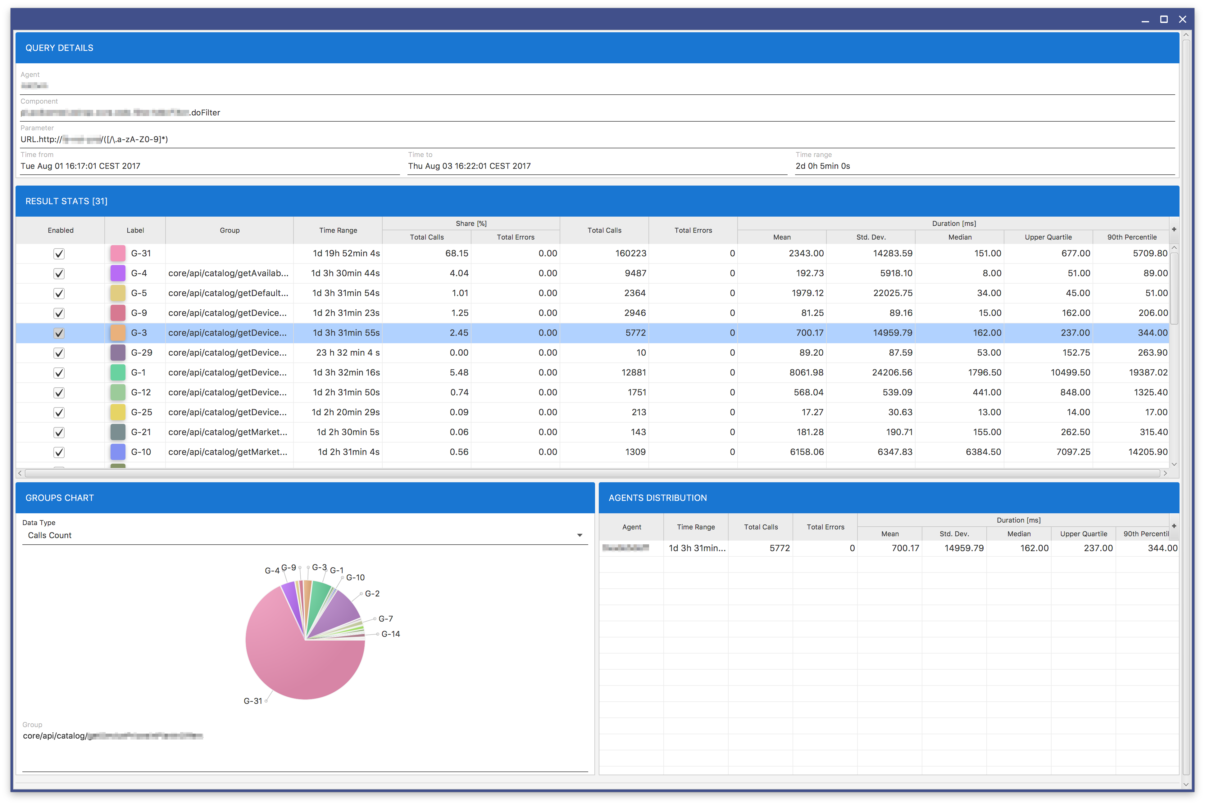
Fig. 8.18 Analytics Result: Group By
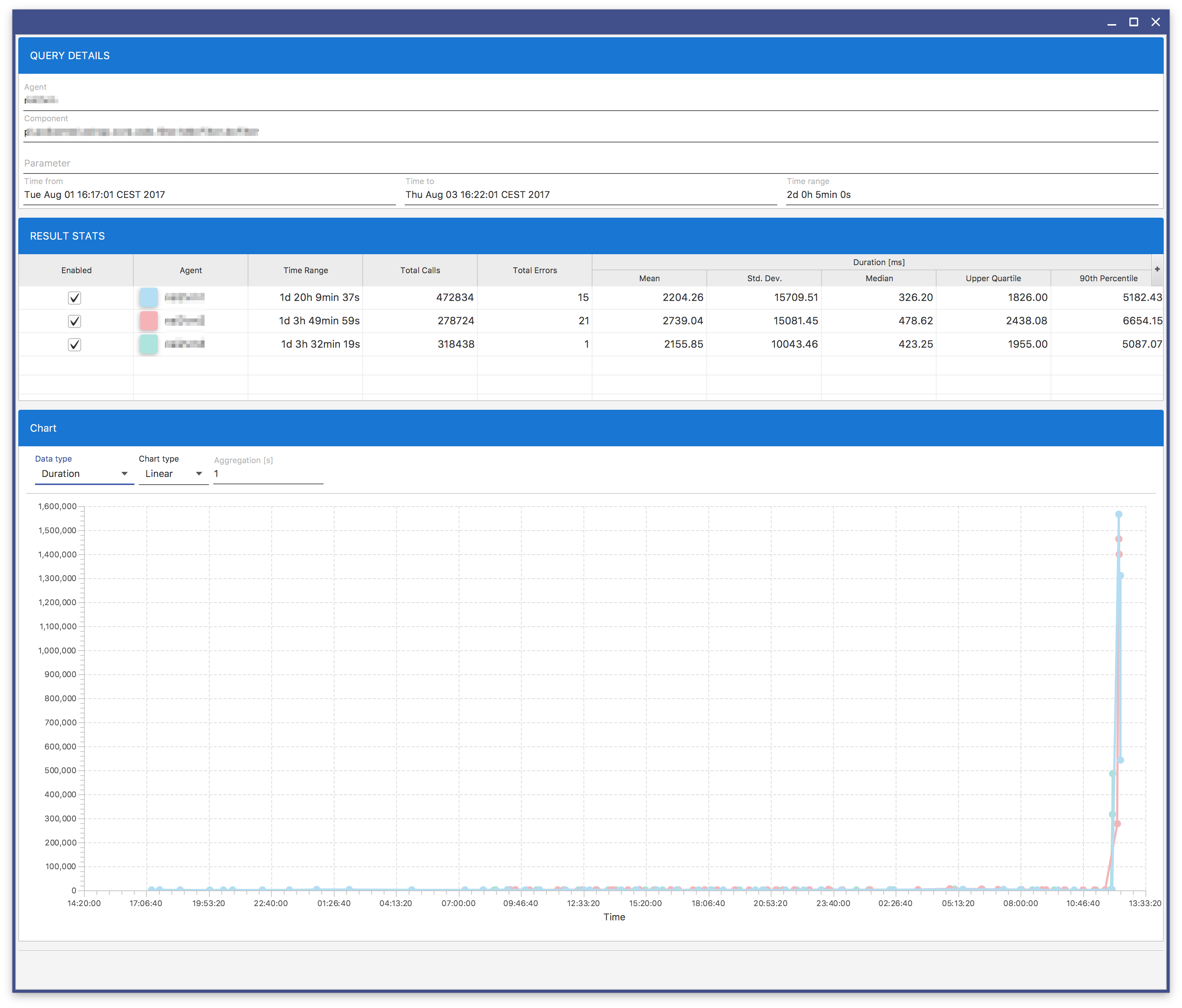
Fig. 8.19 Analytics Result: Duration Graph
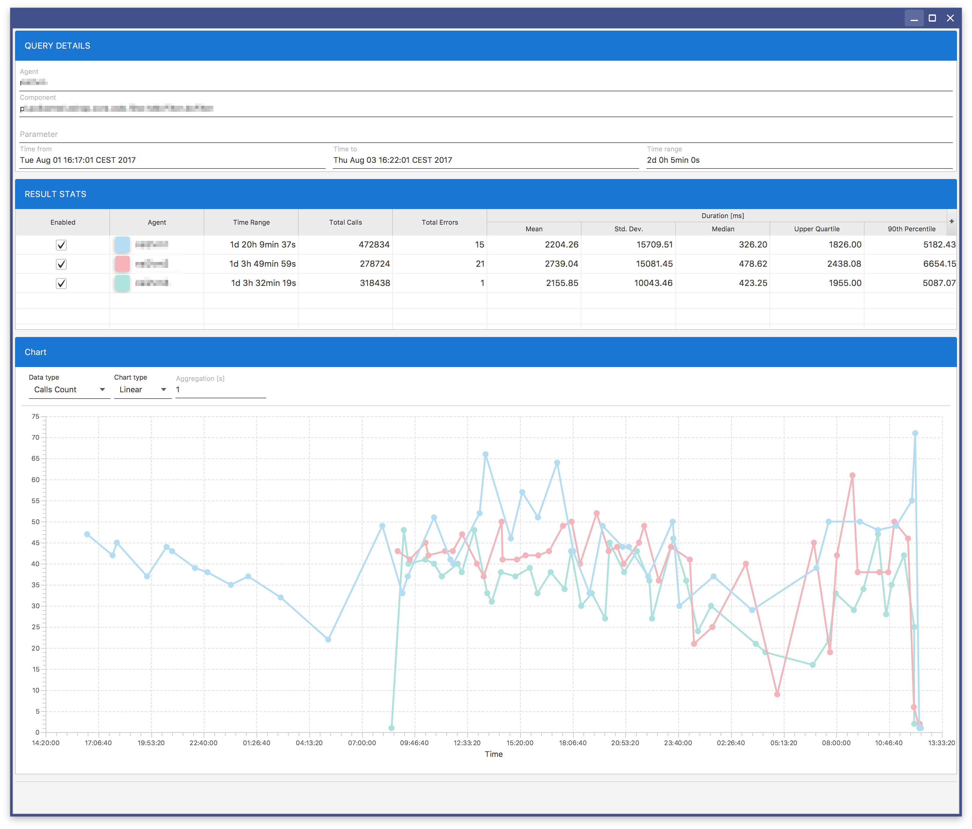
Fig. 8.20 Analytics Result: Calls Graph
8.6. Transactions
This query retrieves a list of transactions and presents it in a table. Use this query if you want to see a detailed view of every transaction executed within the specified time range. The query requires you to fill out the Fig. 8.21 form.
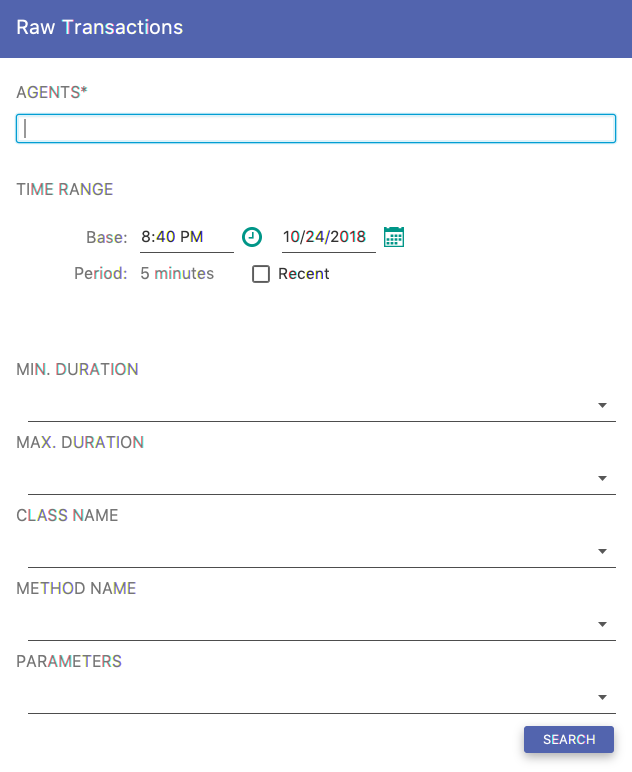
Fig. 8.21 Instrumentation Expanded Form
There are optional fields you can use to narrow down your search results. The DURATION enables you to specify a duration range. In the CLASS NAME entry you can specify a regular expression pattern for a class name. In the METHOD NAME entry you can specify a regular expression pattern for a method name, and finally in the PARAMETERS entry you can set a regular expression for a parameter.
When you click the SEARCH button, you should see a similar view to Fig. 8.22.
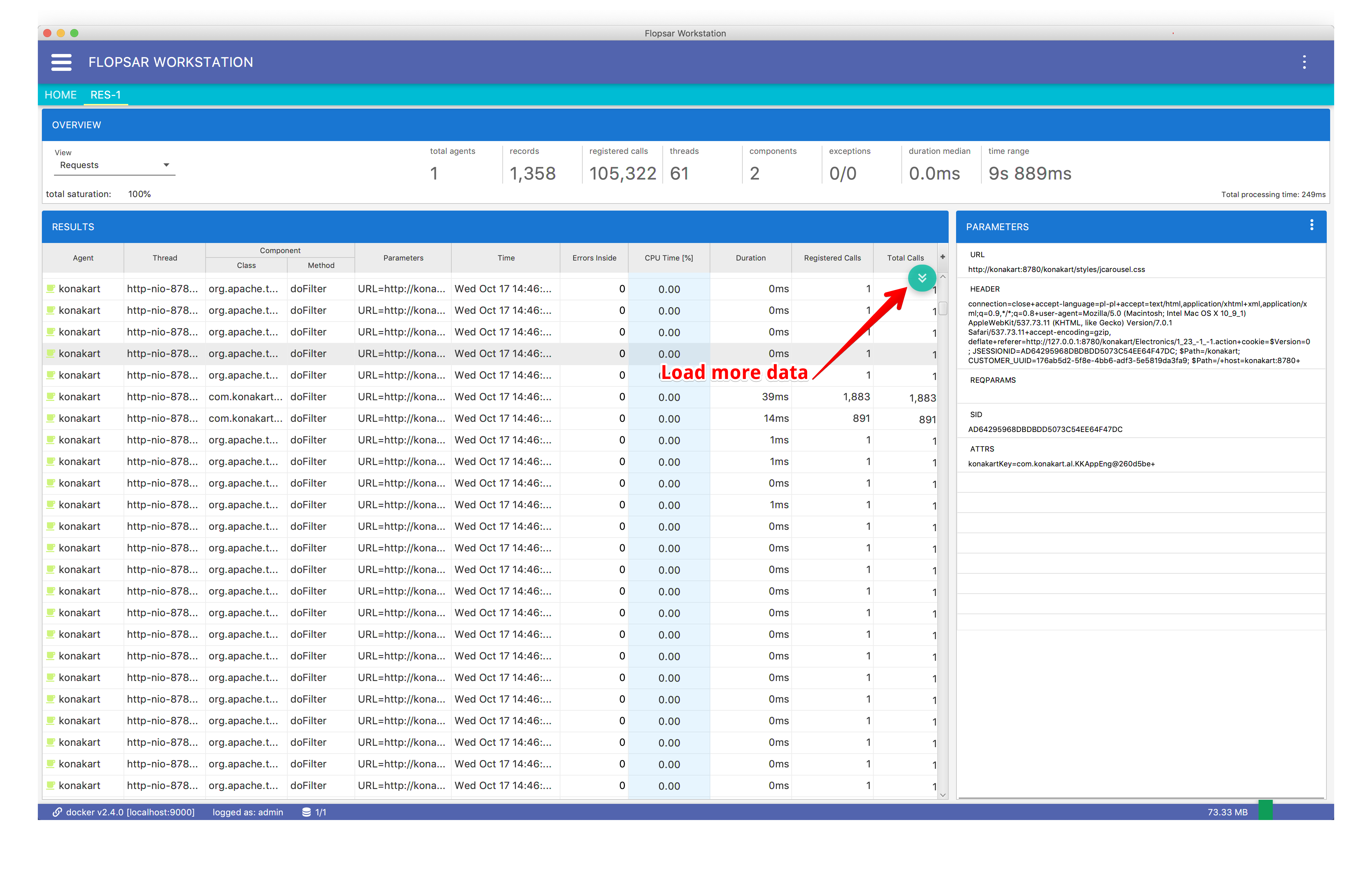
Fig. 8.22 Table results: Records View
Each time when you search instrumentation data you receive only a part of the response data. If you get more, you must click the Load More Data button. You can repeat this procedure to receive more data until the button disappears.
8.6.1. Execution Stack Interpretation
When you double-click some selected record in table Fig. 8.22, you will get a window Fig. 8.23 with this record details. The window presents a tree representing an execution stack of the selected method call. This tree view is self-explanatory but there can be situations where this view can be a bit confusing. This can happen when the displayed execution stack does not exactly correspond to the execution flow you see in your application source code. In order to understand why this situation takes place you must understand how the execution stack tree is built.
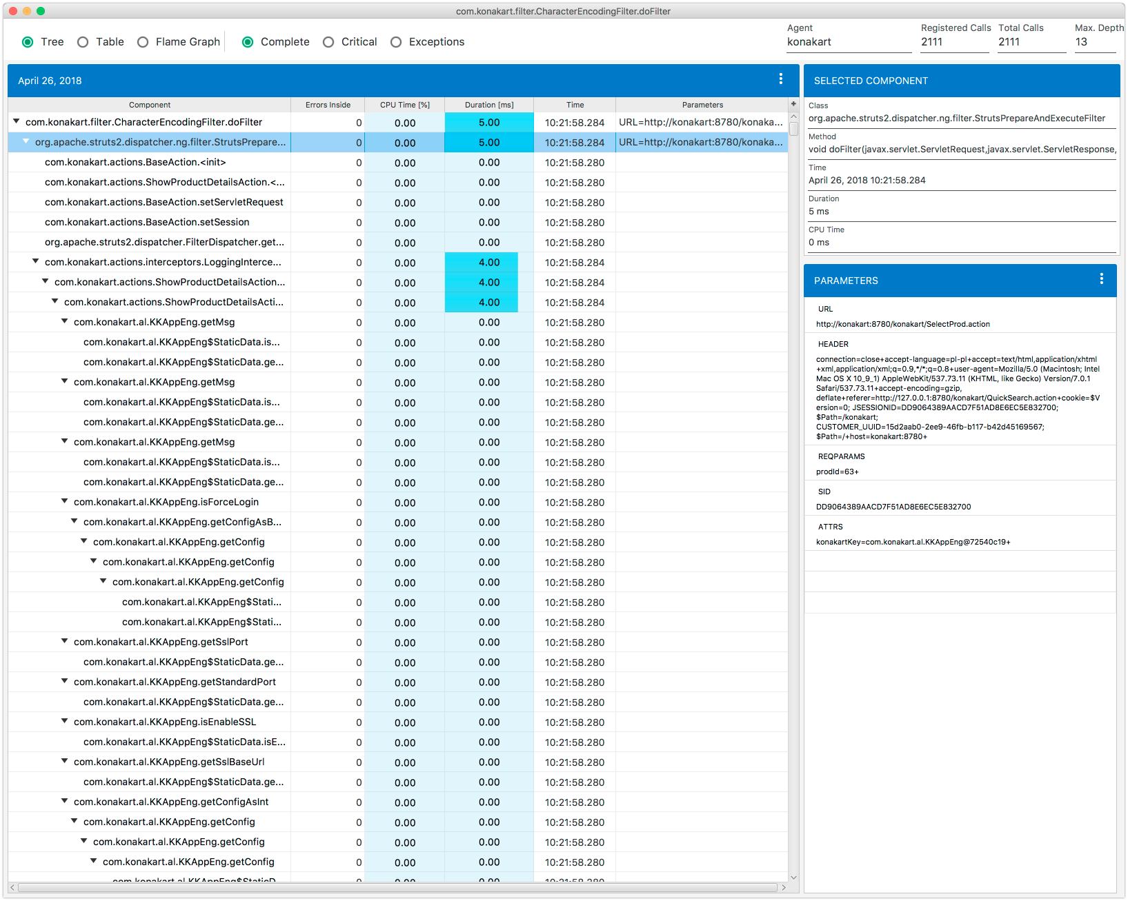
Fig. 8.23 Execution Stack
Note
CPU Time column values are calculated as CPU percentage usage with respect to the corresponding duration value.
If you want to know the exact location of a method call within the execution stack, you can select the Elements Position in the tree options on the stack details. Next time, you expand a branch on the execution stack you should see the positions of methods Fig. 8.24. The position is determined by two numbers, the first one denotes the sequence number within the stack and the second one denotes the stack depth.
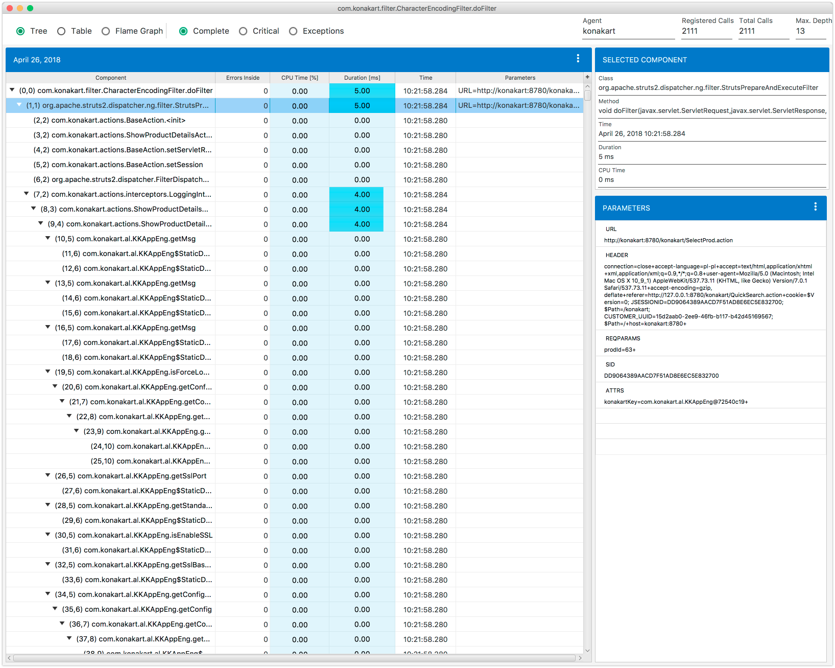
Fig. 8.24 Execution Stack: Methods Calls Position
When you select the Table item, you will get a spectrum view Fig. 8.25. This view presents a spectrum of the execution stack, in other words it shows a collection of all the components which constitute the stack along with their calls and errors statistics.
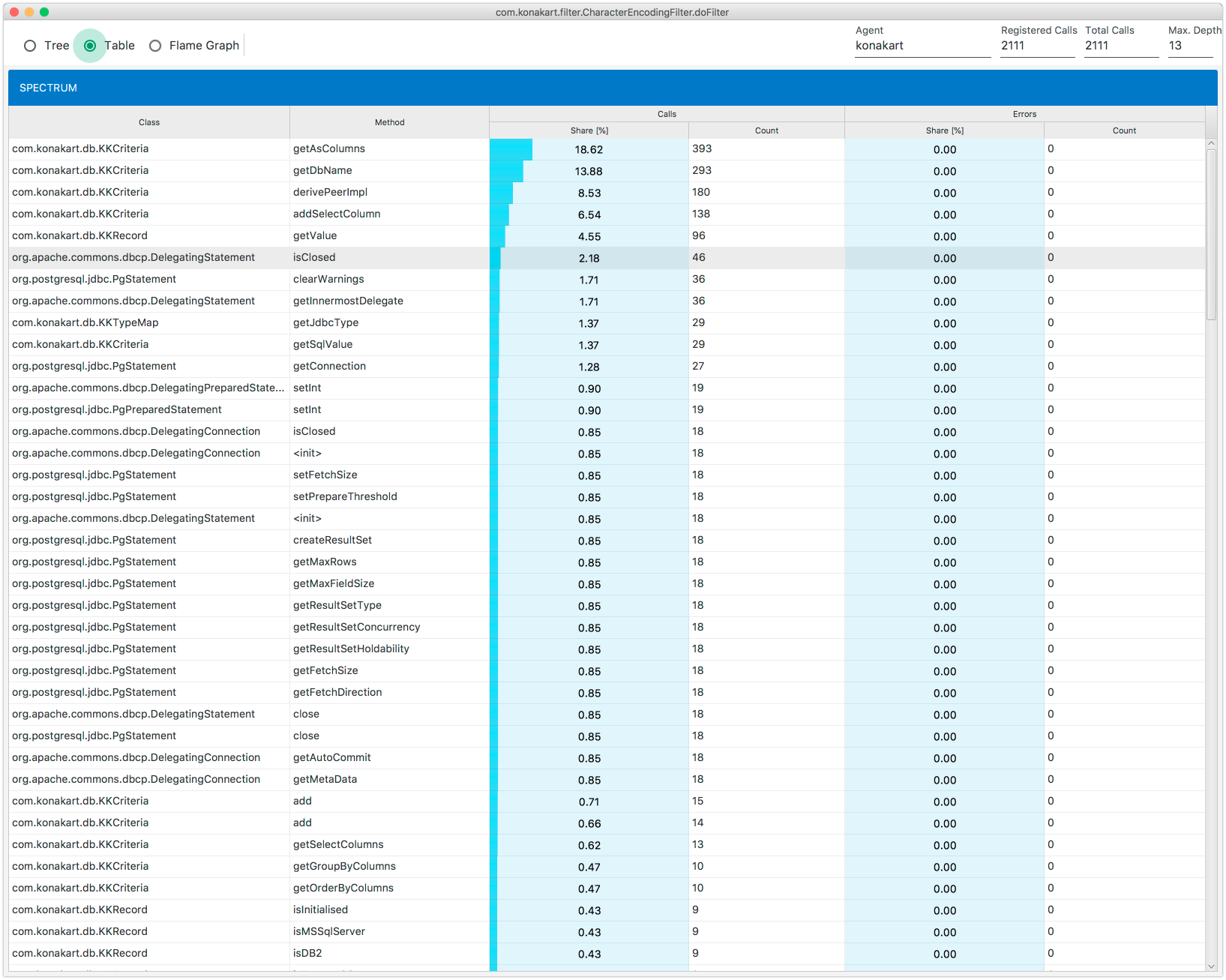
Fig. 8.25 Execution Stack: Spectrum
When you select the Flame Graph item, you will get the Flame Graph view Fig. 8.26.
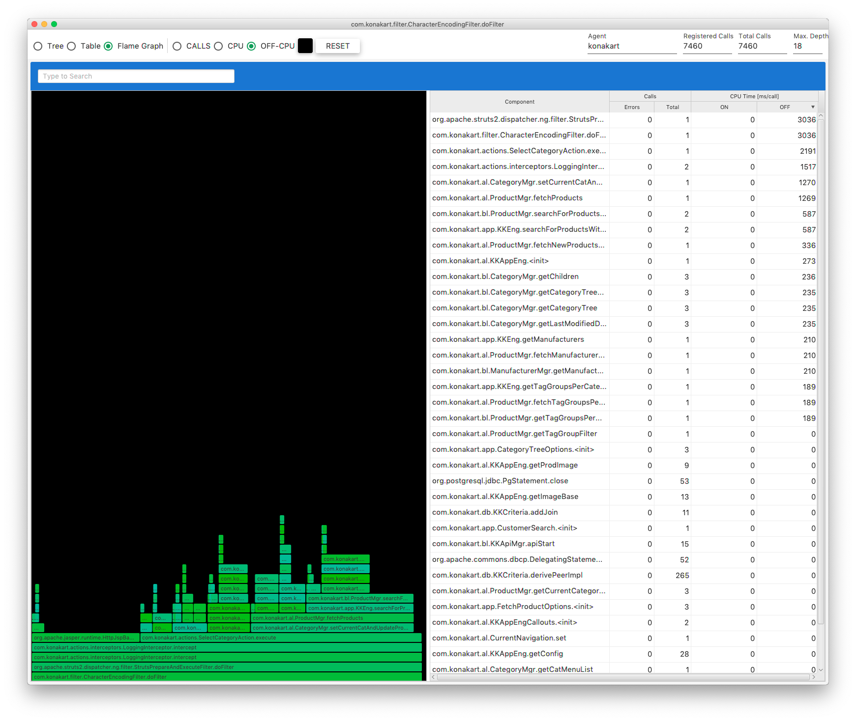
Fig. 8.26 Execution Stack: Flame Graph
In Fig. 8.27 picture you can see four, sample execution stacks of some A method call.
Note
The first method in the execution stack we call a transaction or root call.
The first a view shows how the real execution stack looks. This is a real execution flow that takes place in your application. The second b view, presents the same stack instrumented by your agent. Depending on your configuration, the instrumentation may not cover the entire stack. The empty, gray boxes represent missed, uninstrumented methods. As you can see, at this very point your instrumented execution flow is not complete. Moreover, in your application runtime there can be situations when some of the instrumented method calls will not be reported (refer to Data Collecting Considerations for details). The empty, red boxes in the third c view represent this situation. Finally, what you actually observe in workstation is the last d view. This view presents an assembled stack with missing calls ignored. Now you know how to interpret the execution stack in workstation and why the resulting stack can differ from the original one.
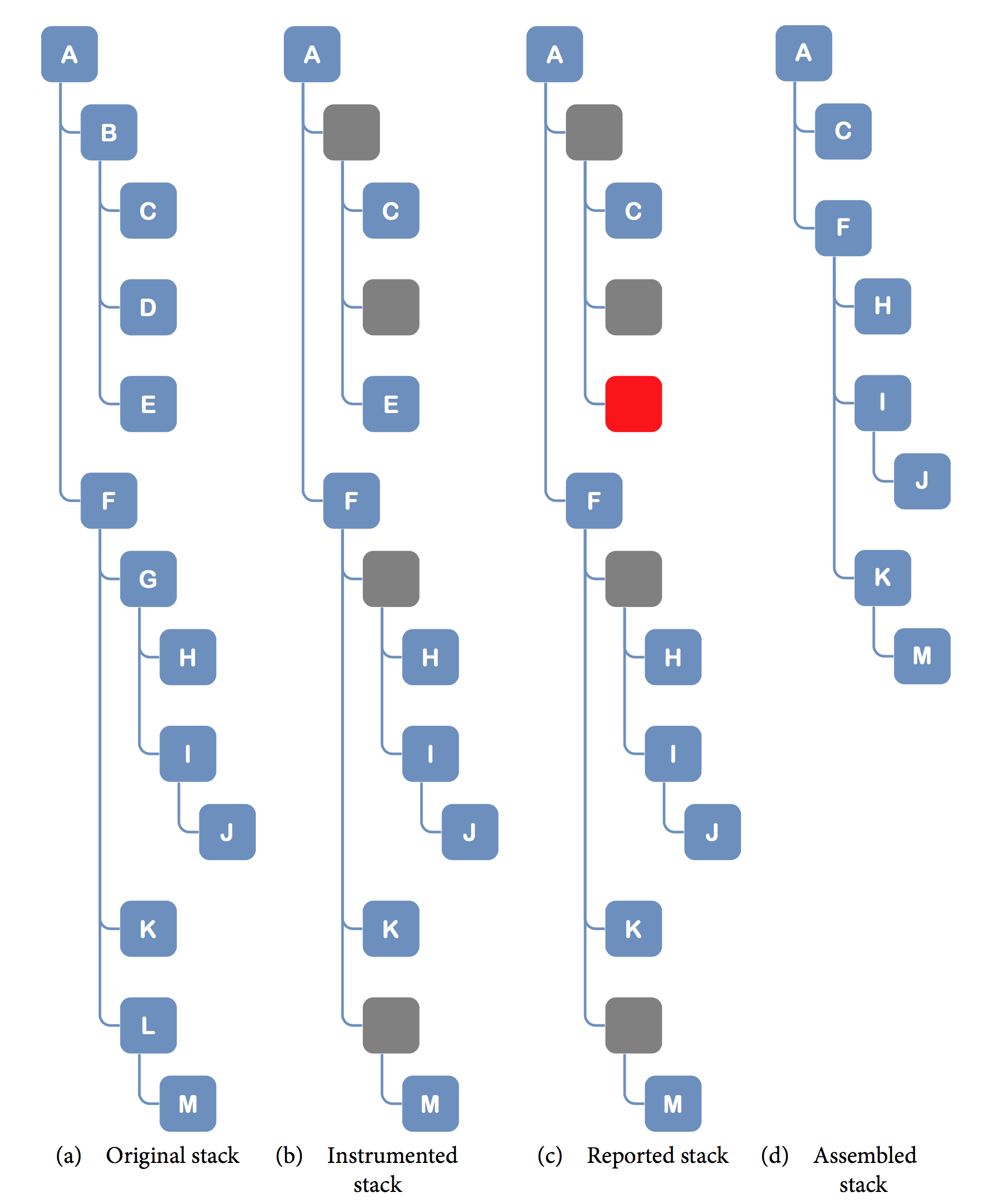
Fig. 8.27 Execution Stack Assembly
8.6.2. Threads Subview
If you want to classify your query results by threads, just select the Threads menu item from the View list in Fig. 8.22 and you will get a view similar to Fig. 8.28.
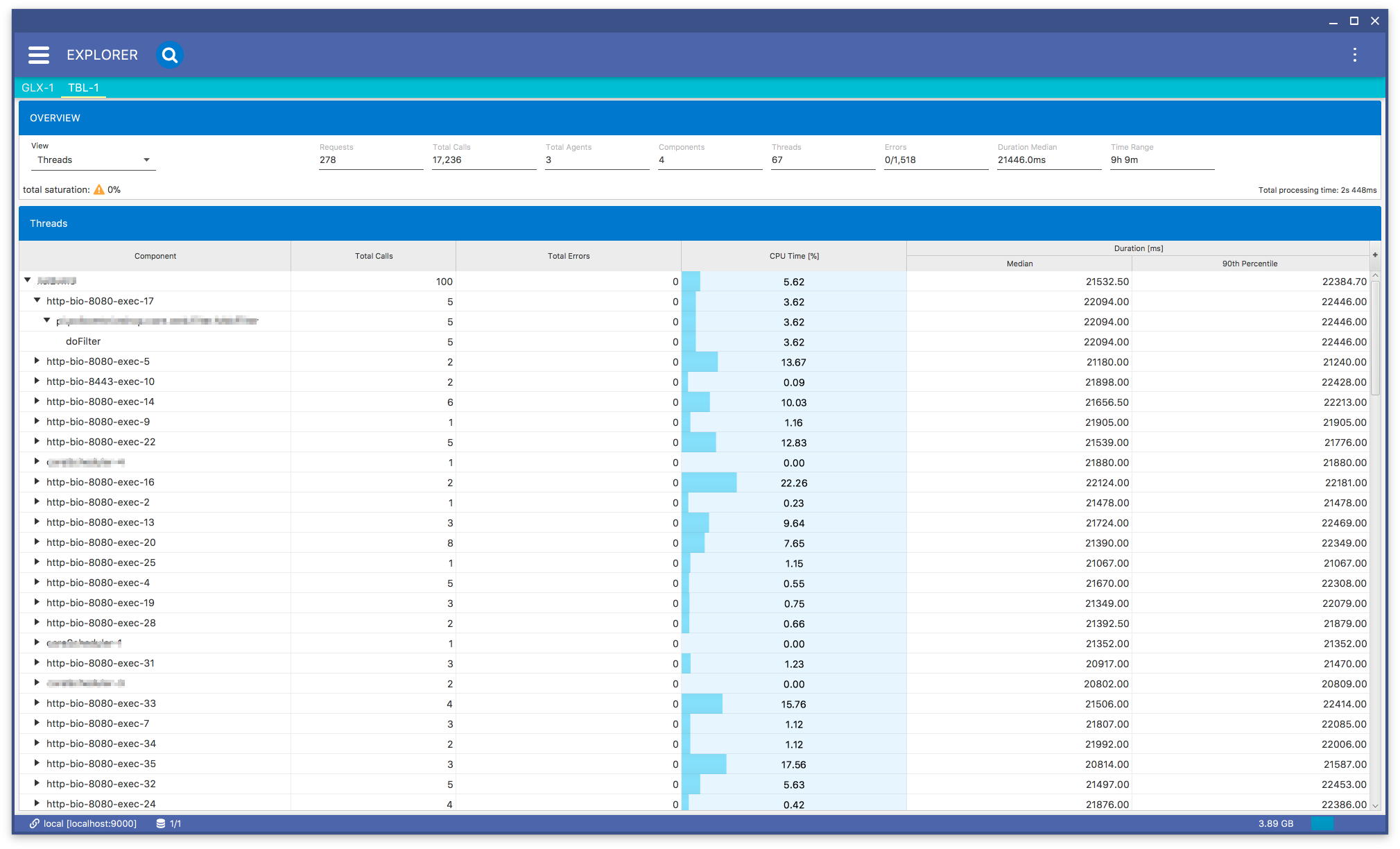
Fig. 8.28 Data Explorer: Threads Subview
The view contains a tree table with the following columns:
| Component: | A tree item, structured as agent –> thread –> class –> method. There are four component levels so the values in each column correspond to the current level. |
|---|---|
| Total Calls: | A total number of calls. |
| Total Errors: | A total number of exceptions thrown. |
| CPU Time: | A total CPU time (if enabled). |
| Duration Median: | |
| A median of duration. | |
| Duration 90th Percentile: | |
| A 90th percentile of duration. | |
8.6.3. Components Subview
When you select the Components menu item in Fig. 8.22 you will get Fig. 8.29 a view:
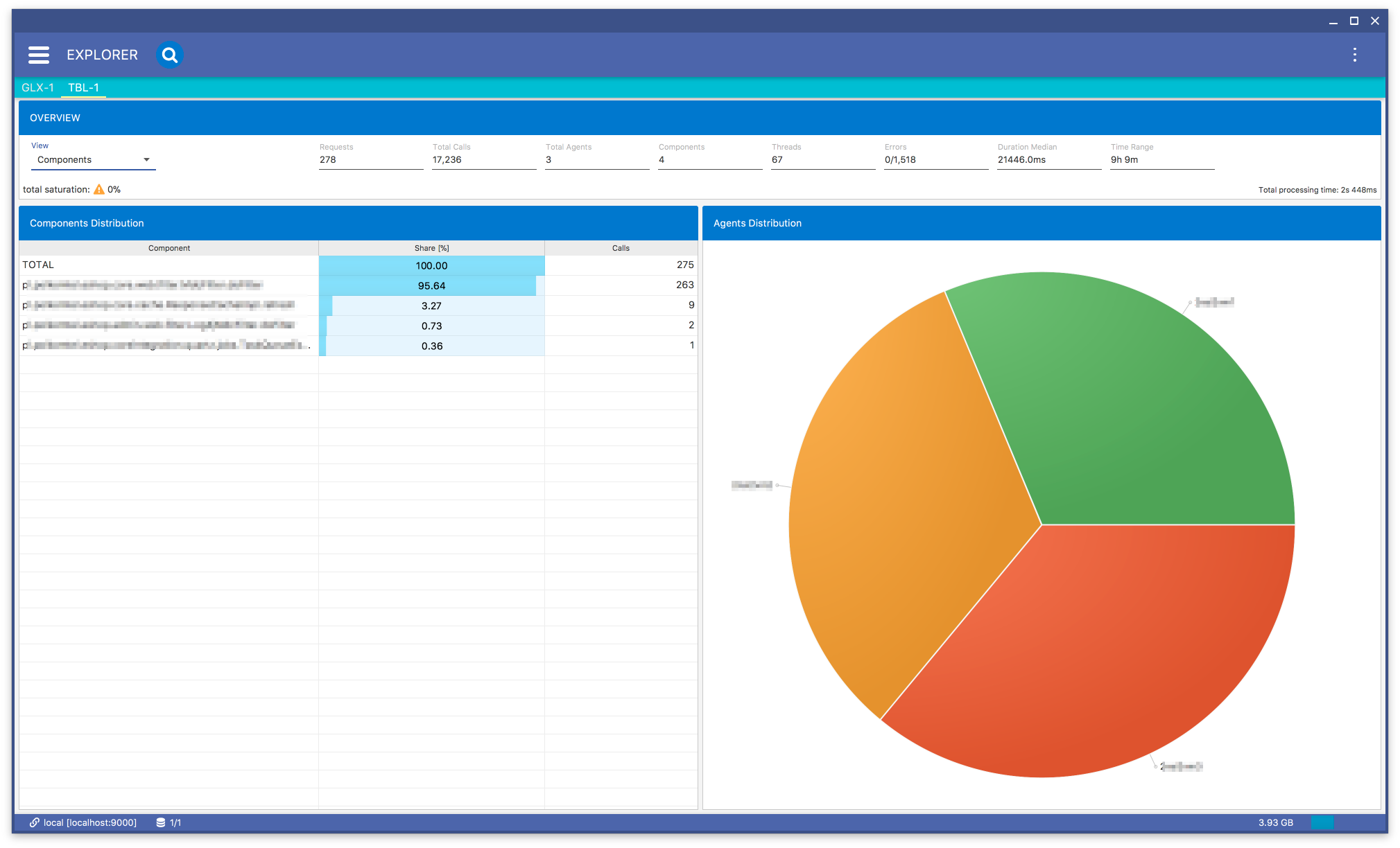
Fig. 8.29 Data Explorer: Components Subview
8.6.4. Errors Subview
When you select the Exceptions menu item in Fig. 8.22 you will get Fig. 8.30 view. In this view you can see what exceptions have been thrown and how their distribution looks like with respect to agents. When you click one of the exceptions you will get its distribution with respect to the agents.
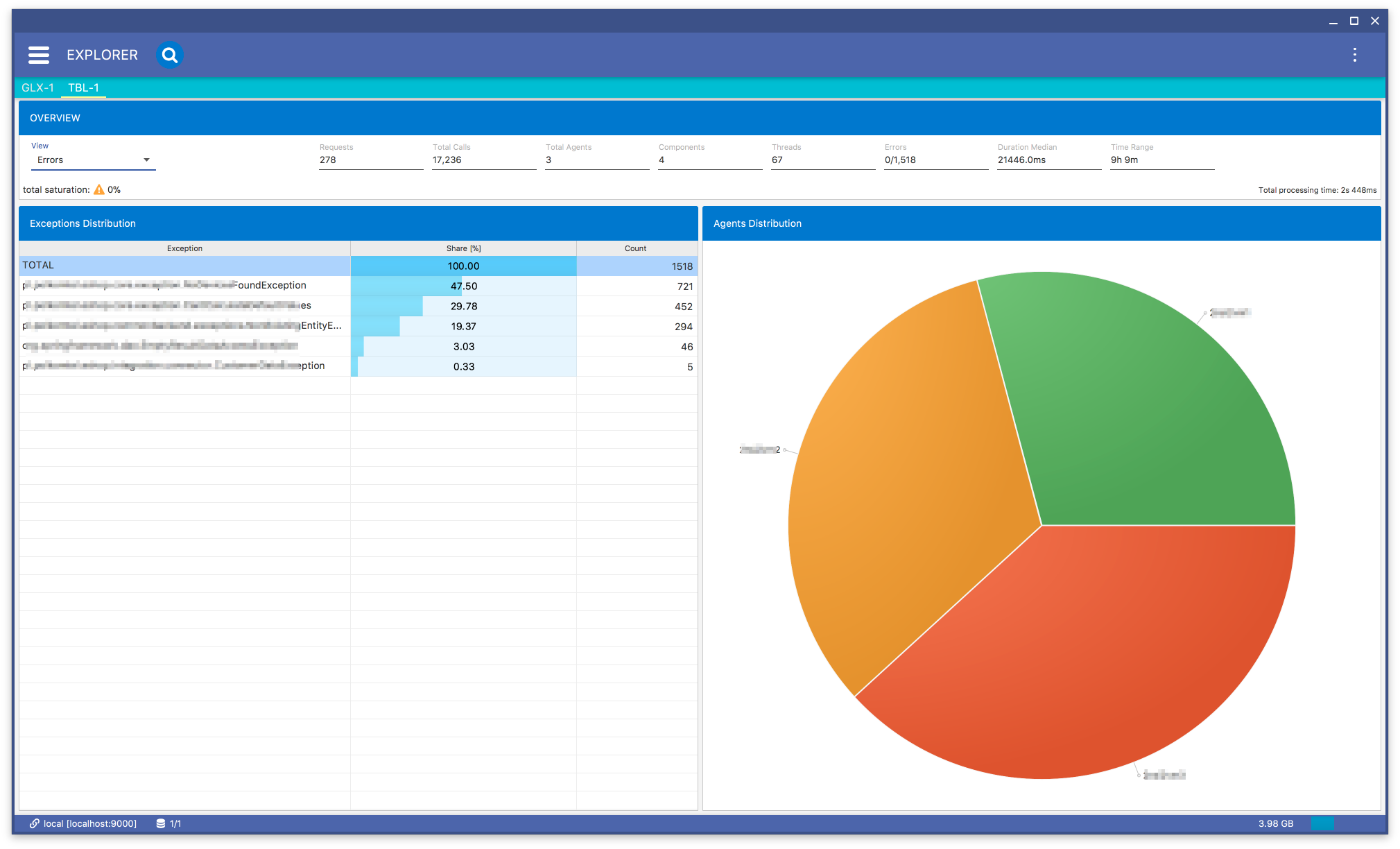
Fig. 8.30 Data Explorer: Errors Subview
8.6.5. Time and Duration Subviews
If you select the Duration Distribution menu item in Fig. 8.22, you will get a bar chart Fig. 8.31 representing a distribution of calls duration. The bars colors correspond to agents.
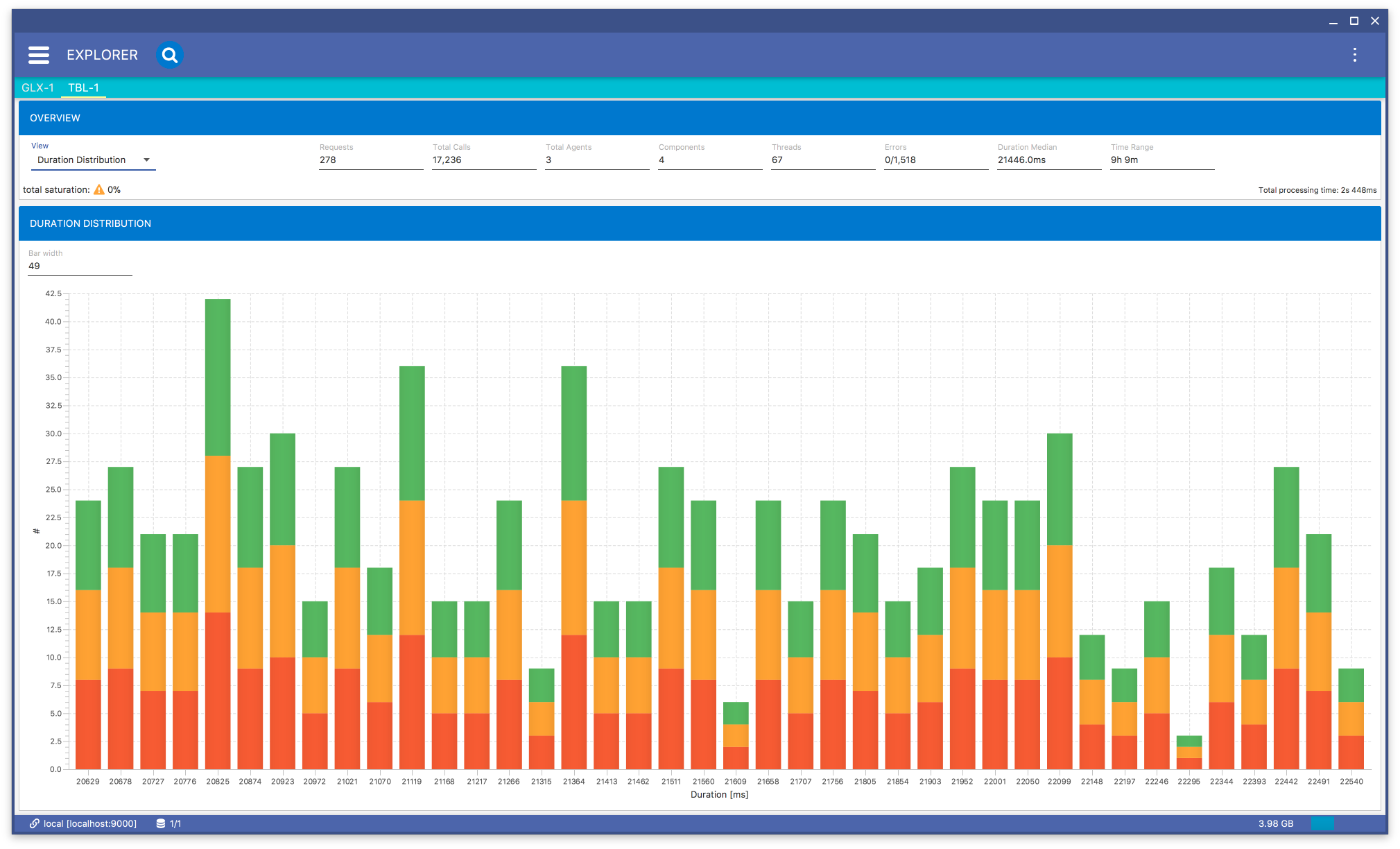
Fig. 8.31 Duration Distribution
If you select the Time Distribution menu item in Fig. 8.22, you will get a bar chart Fig. 8.32 representing a distribution of calls count. The bars colors correspond to agents.
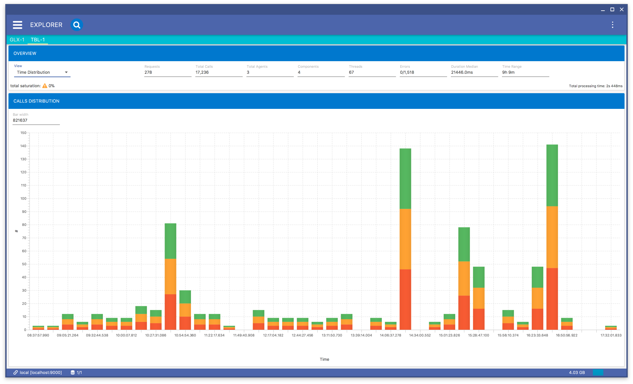
Fig. 8.32 Calls Distribution
8.7. Threads Dump
This query retrives a thread dump from agents, whose names match the specified agents’ pattern. You can use this query only for currently connected agents do the manager.

Fig. 8.33 Thread Dump Form
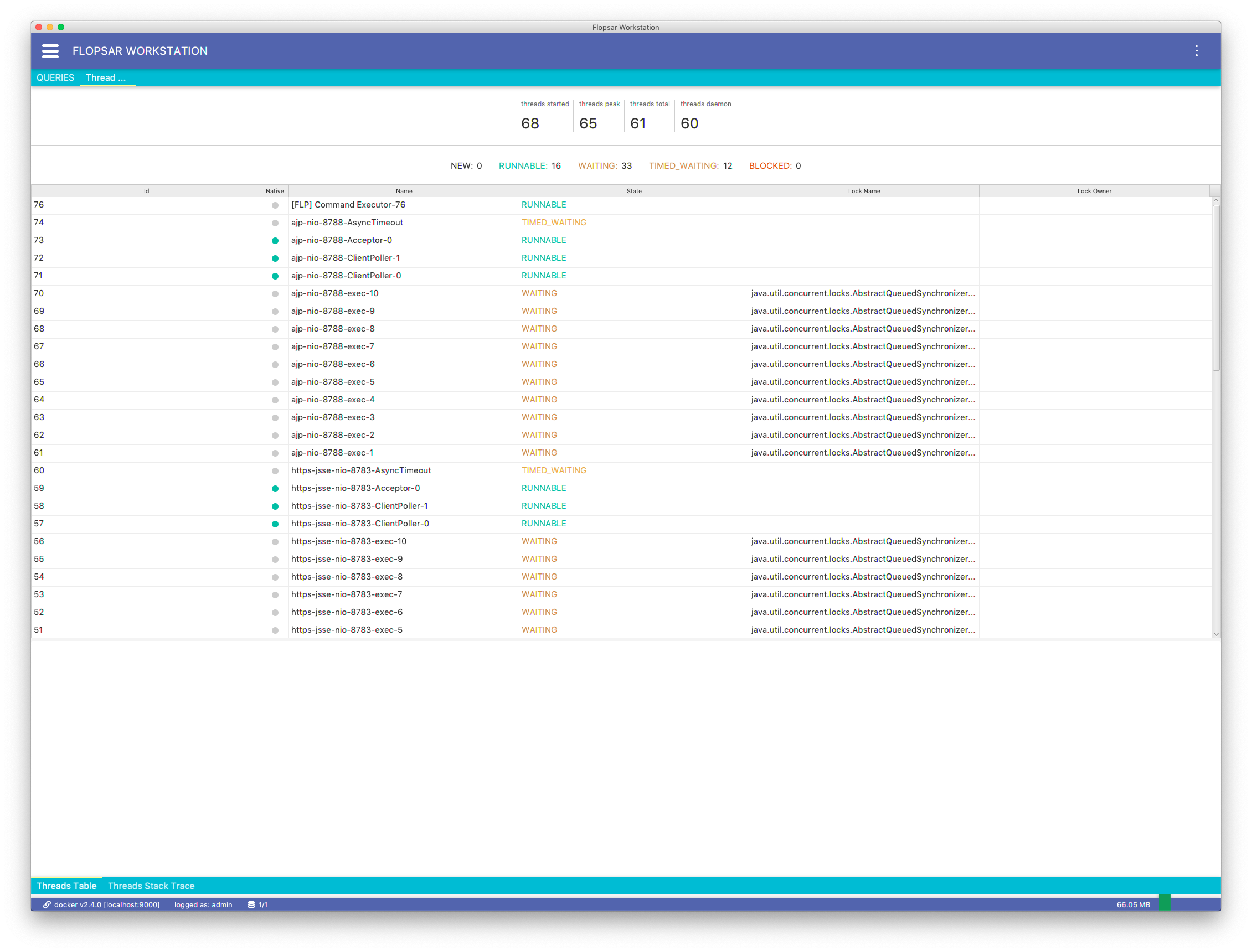
Fig. 8.34 Threads Dump: Threads
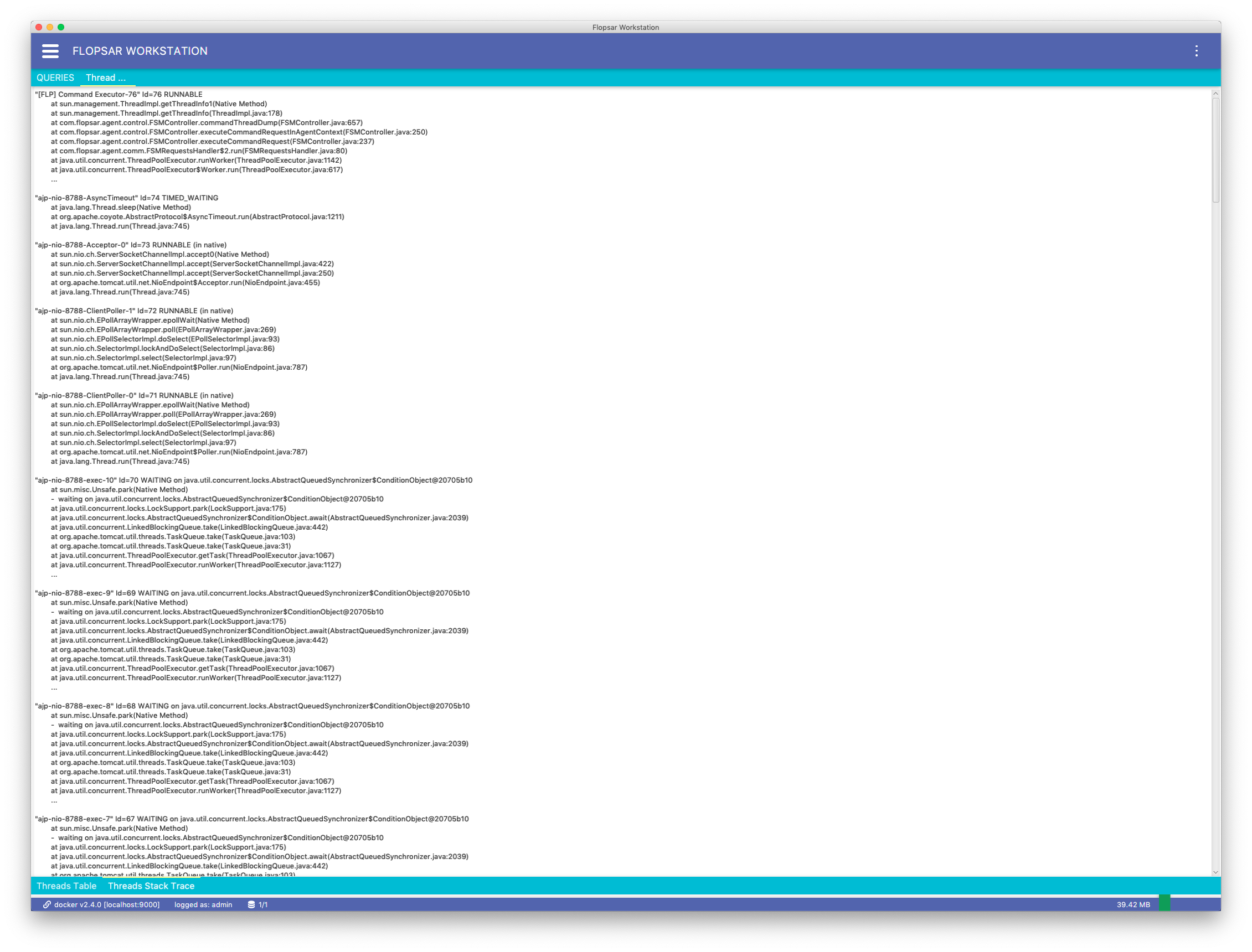
Fig. 8.35 Threads Dump: Details
8.8. Top 30 Exceptions
This query retrieves top 30 exceptions thrown within some particular time range.
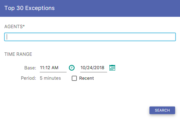
Fig. 8.36 Top 30 Exceptions Form
As a result you should obtain a similar view to the one below:
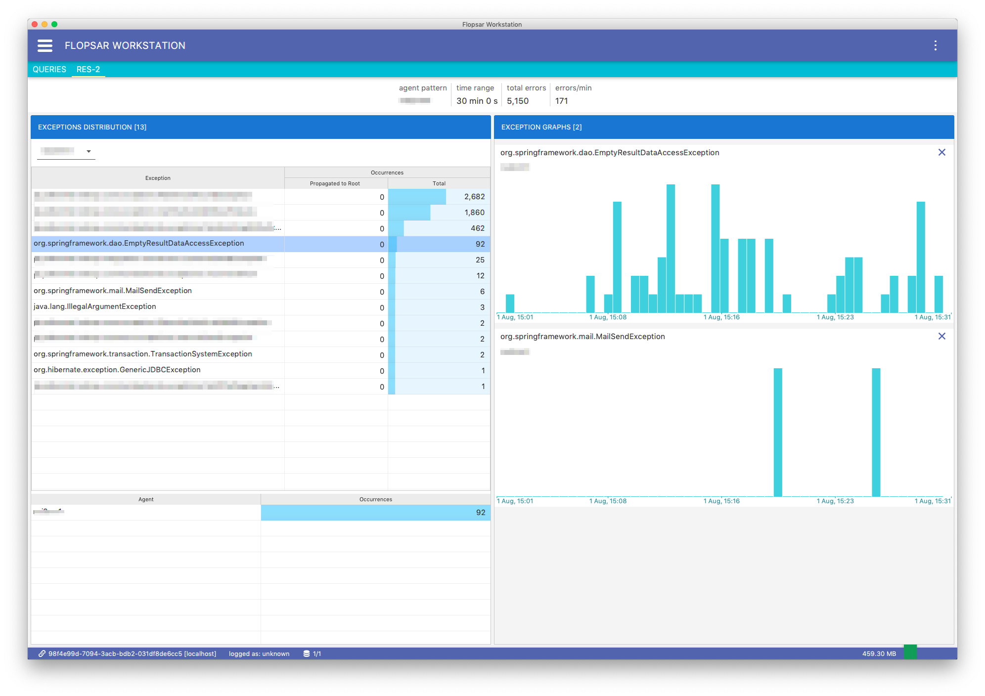
Fig. 8.37 Exceptions Analysis
This view presents a top 30 list of thrown exceptions. The top bar contains the following information:
| agent pattern: | Agent pattern used to query the data. |
|---|---|
| time range: | Time range the data come from. |
| total errors: | Total number of exceptions. |
| errors/min: | Average number of exceptions thrown per minute. |
There is a table for each found agent. The table consists of three columns:
| Exception: | Exception class. |
|---|---|
| Occurrences - Propagated to Root: | |
| Number of exceptions, which propagated to the root call. If this number is zero, it means that all the exceptions have been handled by the application. | |
| Occurrences - Total: | |
| Number of exceptions. | |
Everytime you select an exception in the table, you get the exception distribution per agent in the second table, right below the one with exceptions.
If you want to know how particular exception occurrences are distributed over time, just select the exception from the table and Occurrences Time Histogram item in the context menu. You will get a bar chart with the selected exception occurrences over time. You can click the bars to see more details.
If you want to see where the selected exception come from, just select Affected Calls item from the context menu.